Classification

Jon Reades

Spot the Difference

On Maps

  • Group observations by ‘class’.
  • Typically based on 1-D distribution.
  • Classes are assigned by user choice.

On Labels

  • Label observations by ‘class’.
  • Typically based on model outputs.
  • Labels are assigned by user feedback.

Map Classification Choices

  • Assign classes manually.
  • Split range evenly.
  • Split data evenly
  • Split data according to distribution
  • Split data according to their similarity to each other.

In Practice…

Mapclassify

Mapclassify (part of PySAL) provides a wide range of classifiers:

No Parameters k Parameter
BoxPlot UserDefined
StdMean Percentiles
MaxP Quantiles
HeadTailBreaks Natural Breaks
EqualInterval Maximum Breaks
JenksCaspall/Sampled/Forced
FisherJenks/Sampled

k will a user-specified number of classes or binning criterion.

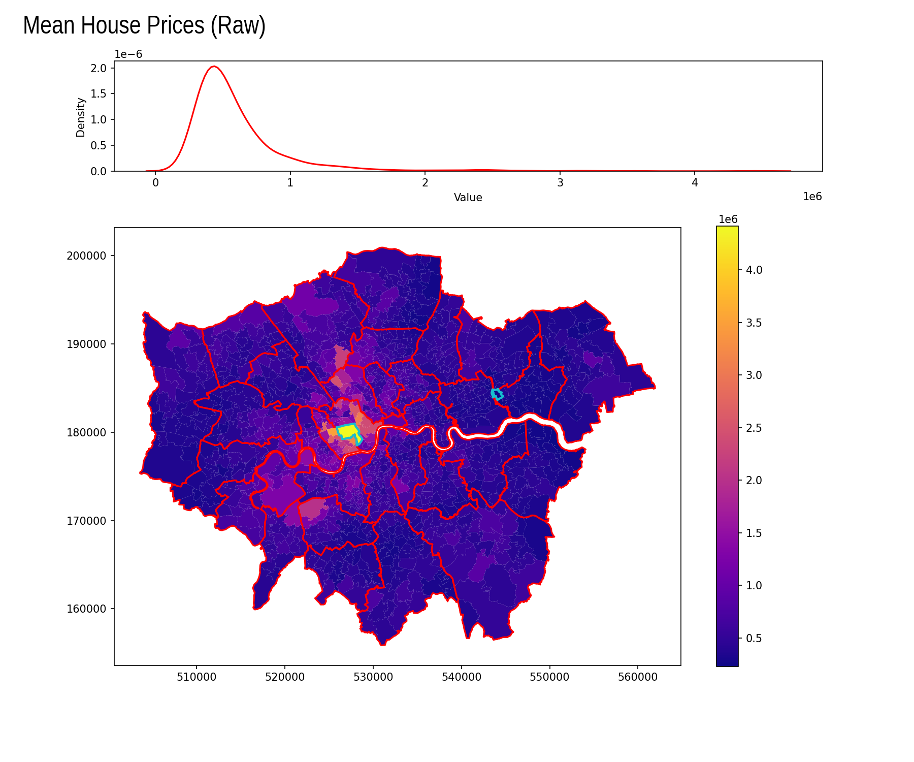
Raw

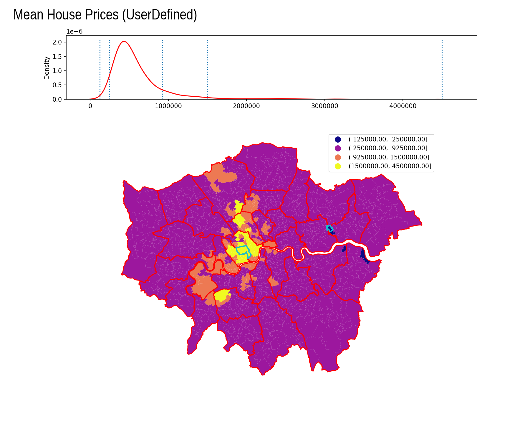
User Defined

Interval Count
( -inf, 125000.00] 0
( 125000.00, 250000.00] 4
( 250000.00, 925000.00] 865
( 925000.00, 1500000.00] 85
(1500000.00, 4500000.00] 29

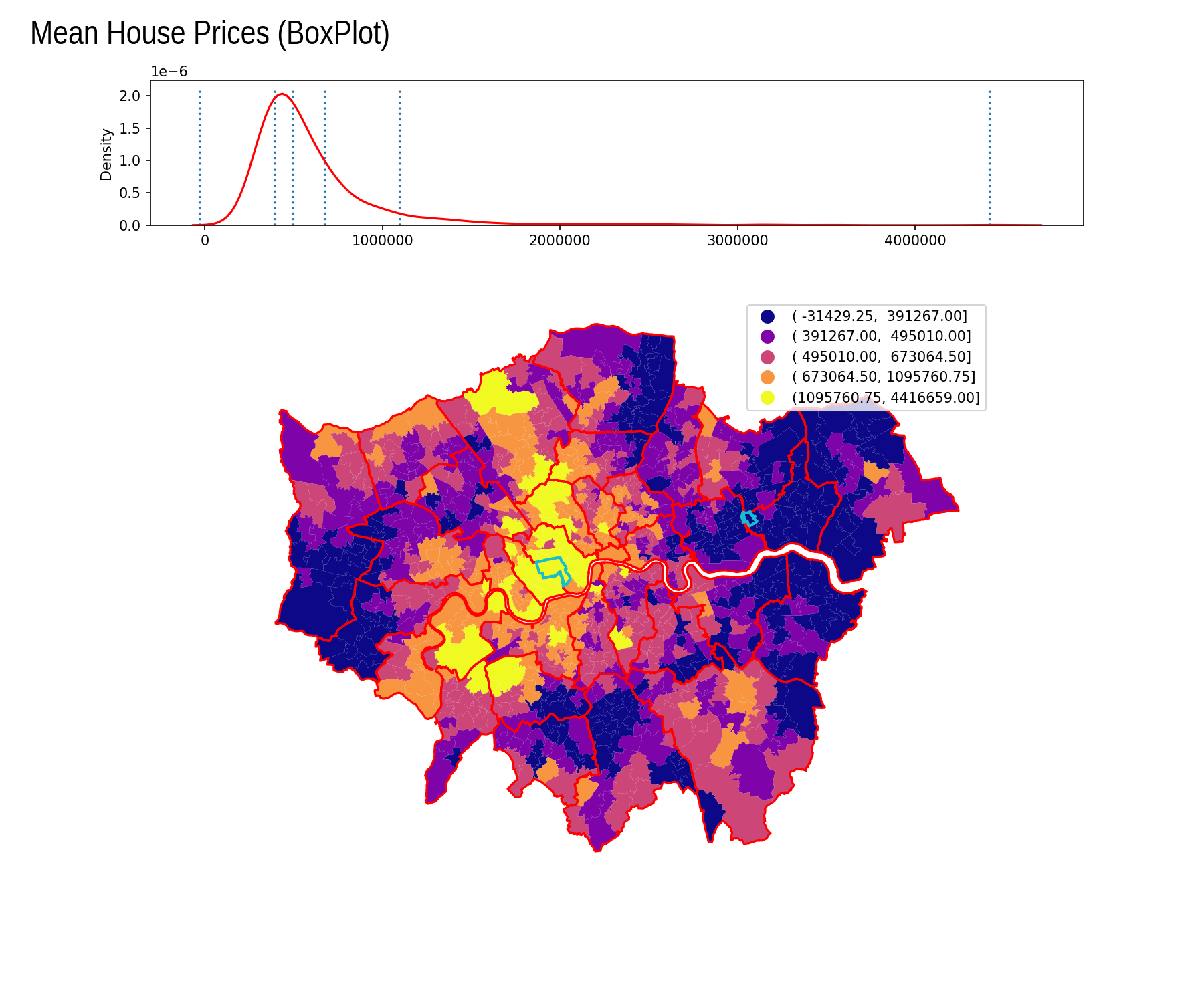
Box Plot

Interval Count
( -inf, -31429.25] 0
( -31429.25, 391267.00] 246
( 391267.00, 495010.00] 246
( 495010.00, 673064.50] 245
( 673064.50, 1095760.75] 175
(1095760.75, 4416659.00] 70

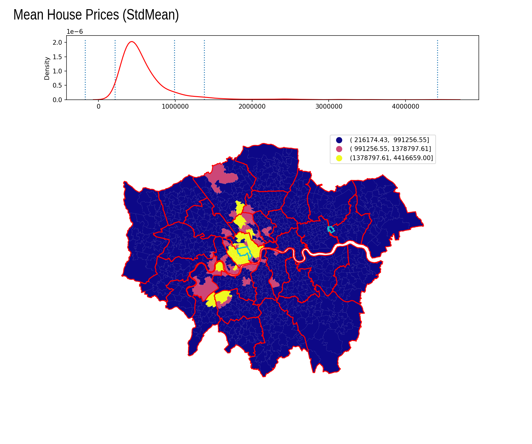
Standard Deviations

Interval Count
( -inf, -171366.63] 0
(-171366.63, 216174.43] 0
( 216174.43, 991256.55] 892
( 991256.55, 1378797.61] 53
(1378797.61, 4416659.00] 38

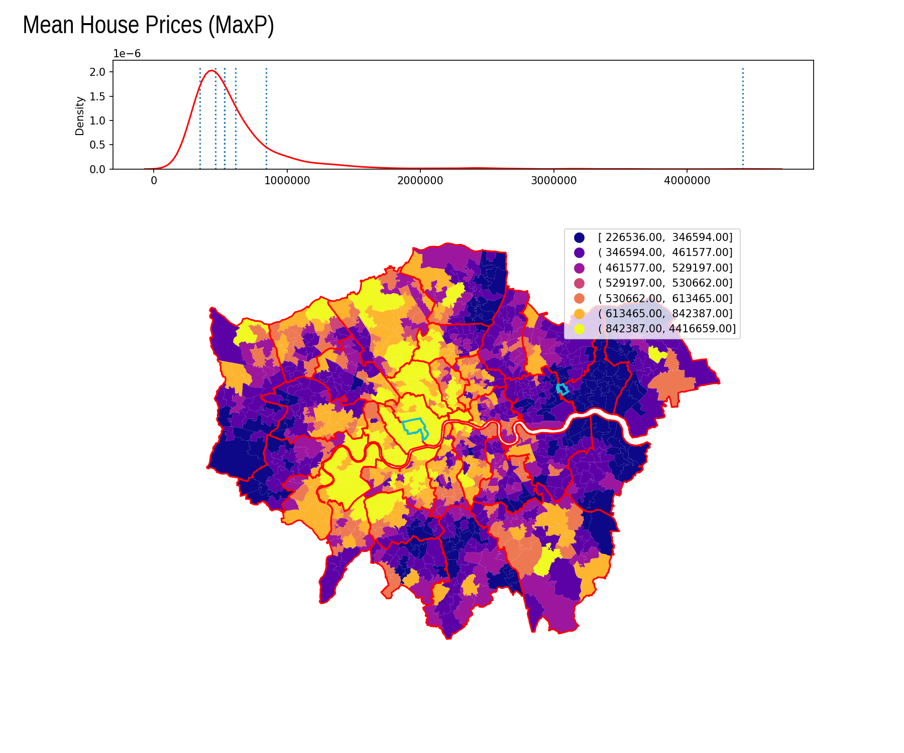
Max P

Interval Count
[ 226536.00, 346594.00] 142
( 346594.00, 461577.00] 279
( 461577.00, 529197.00] 140
( 529197.00, 530662.00] 3
( 530662.00, 613465.00] 115
( 613465.00, 842387.00] 167
( 842387.00, 4416659.00] 137

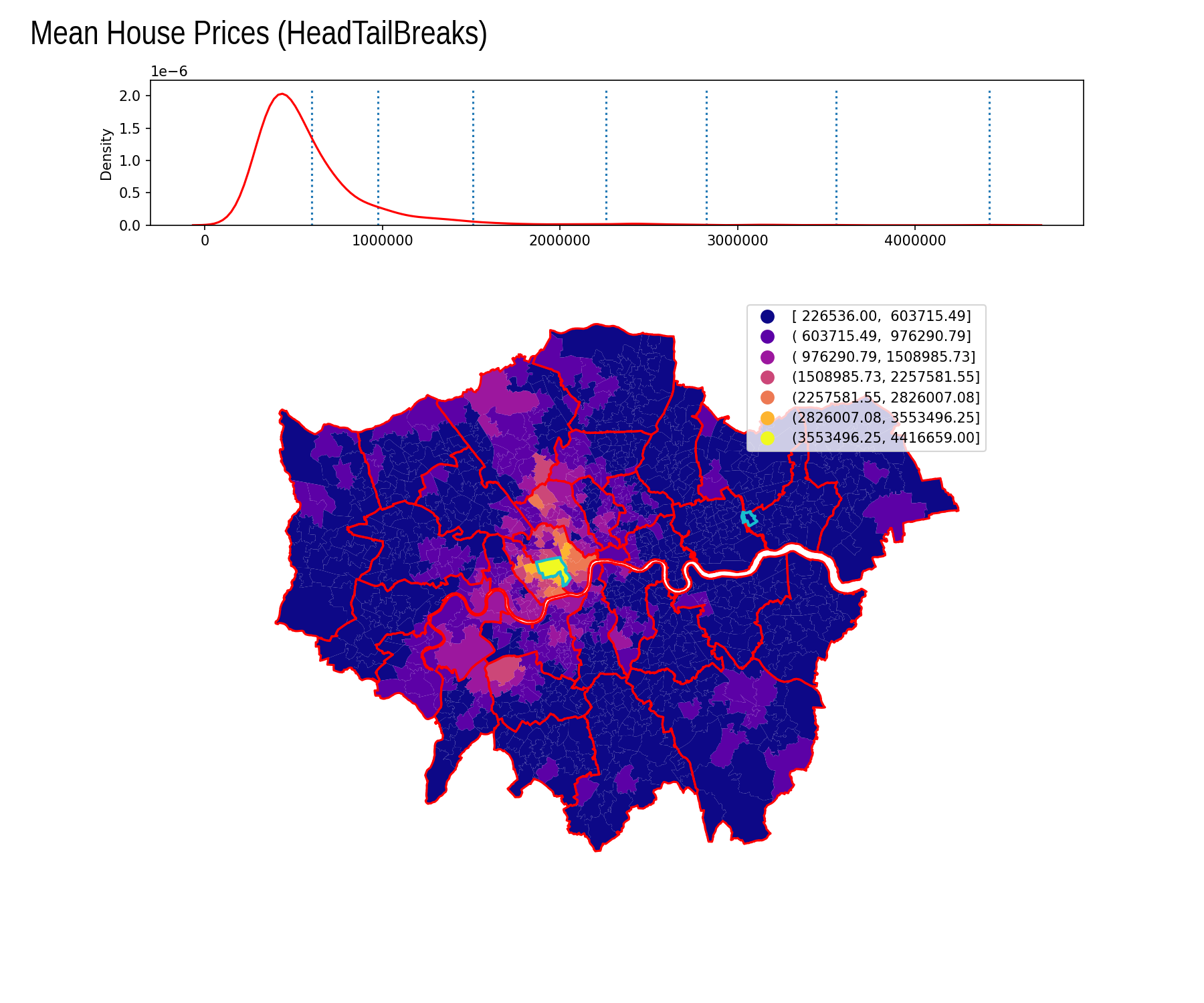
Head Tail Breaks

Interval Count
[ 226536.00, 603715.49] 670
( 603715.49, 976290.79] 218
( 976290.79, 1508985.73] 66
(1508985.73, 2257581.55] 16
(2257581.55, 2826007.08] 9
(2826007.08, 3553496.25] 3
(3553496.25, 4416659.00] 1

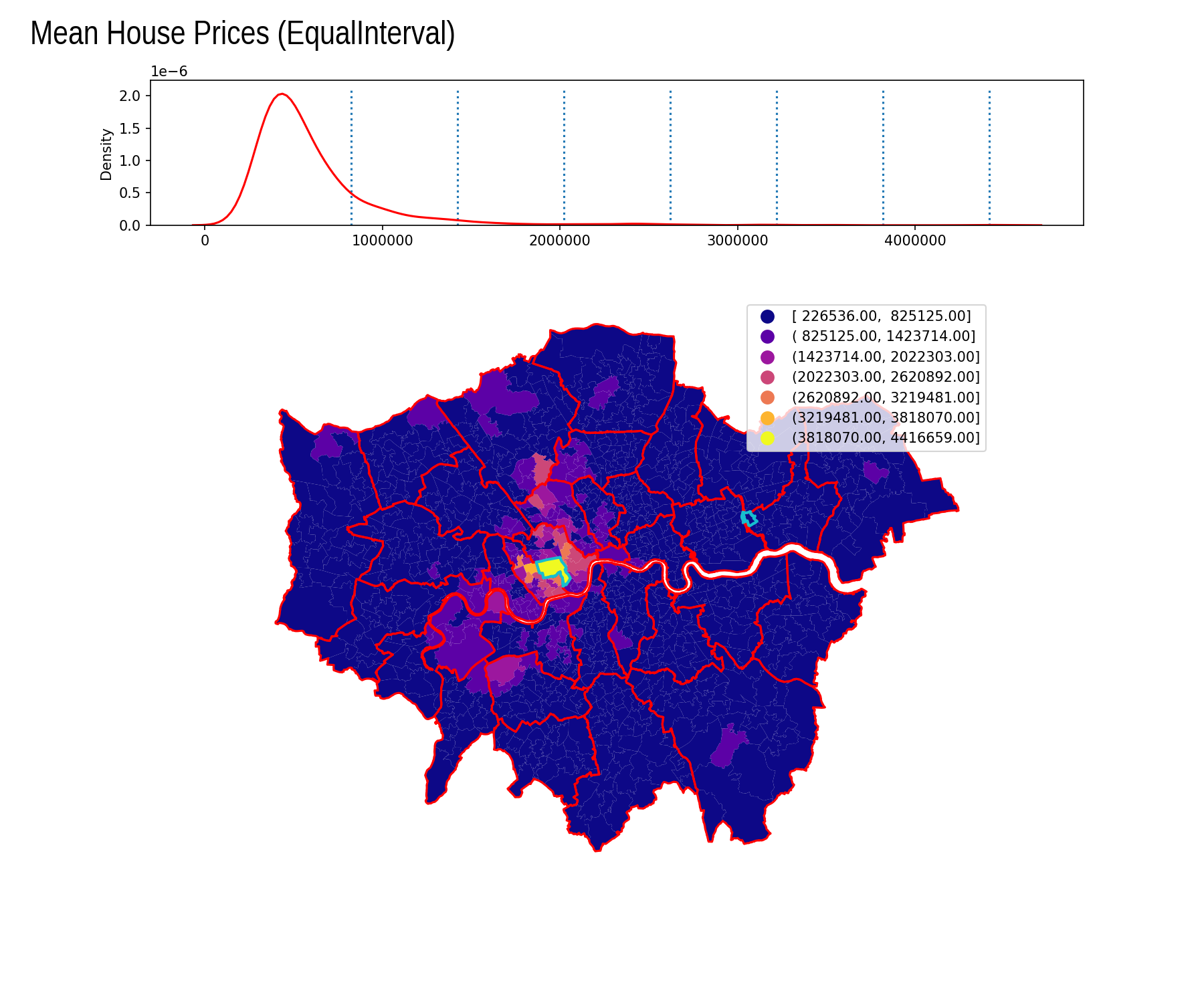
Equal Interval

Interval Count
[ 226536.00, 825125.00] 842
( 825125.00, 1423714.00] 108
(1423714.00, 2022303.00] 17
(2022303.00, 2620892.00] 10
(2620892.00, 3219481.00] 4
(3219481.00, 3818070.00] 1
(3818070.00, 4416659.00] 1

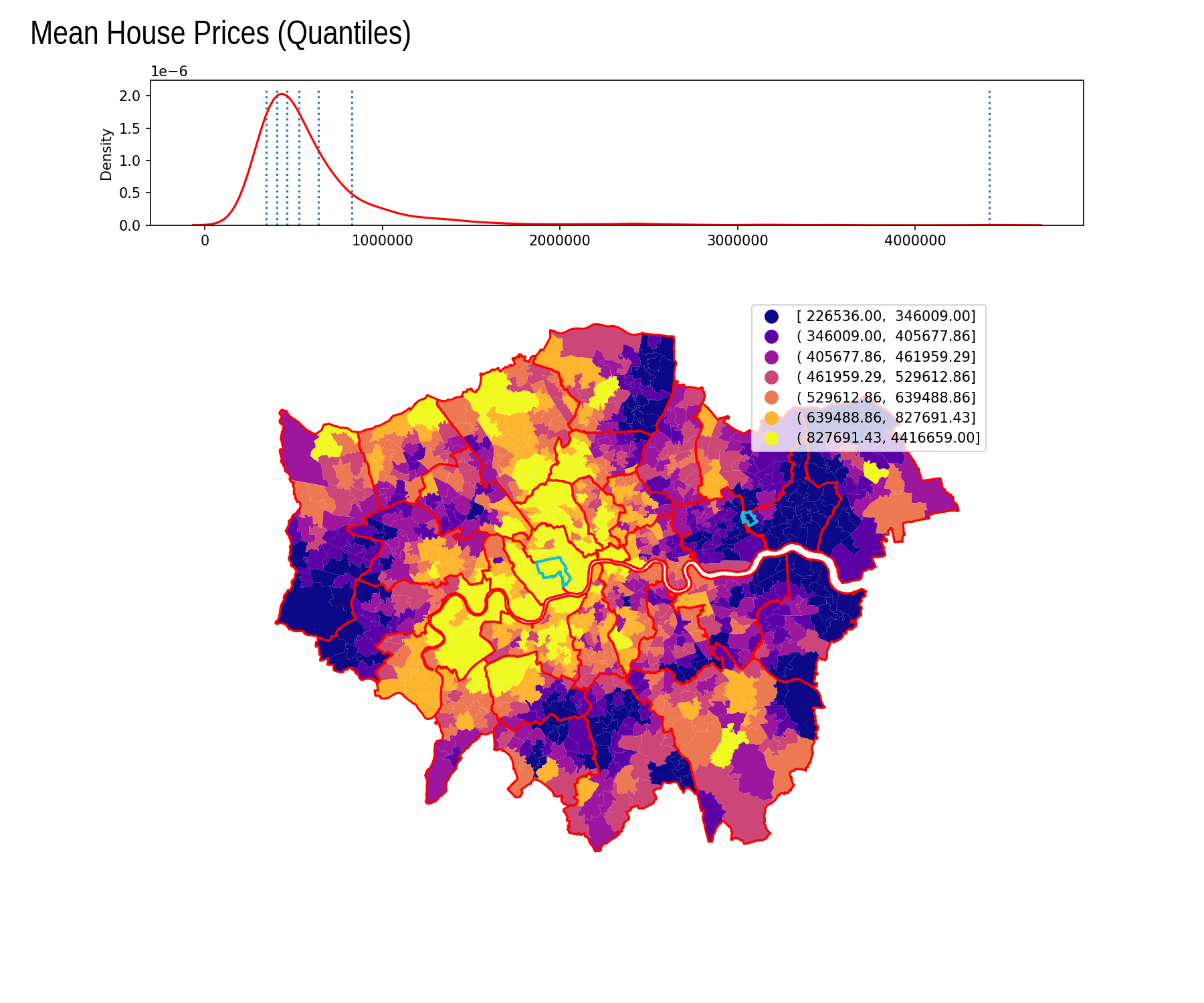
Quantiles

Interval Count
[ 226536.00, 346009.00] 140
( 346009.00, 405677.86] 140
( 405677.86, 461959.29] 140
( 461959.29, 529612.86] 141
( 529612.86, 639488.86] 140
( 639488.86, 827691.43] 140
( 827691.43, 4416659.00] 141

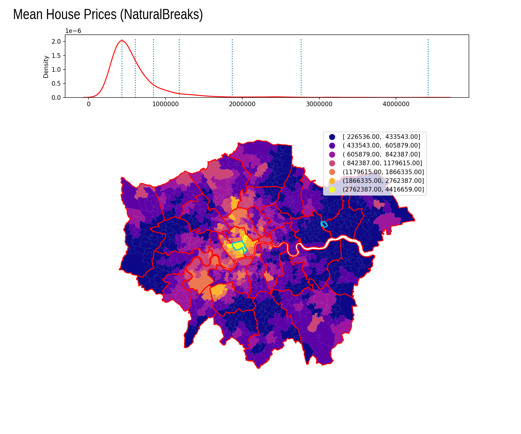
Natural Breaks

Interval Count
[ 226536.00, 433543.00] 356
( 433543.00, 605879.00] 316
( 605879.00, 842387.00] 174
( 842387.00, 1179615.00] 80
(1179615.00, 1866335.00] 39
(1866335.00, 2762387.00] 14
(2762387.00, 4416659.00] 4

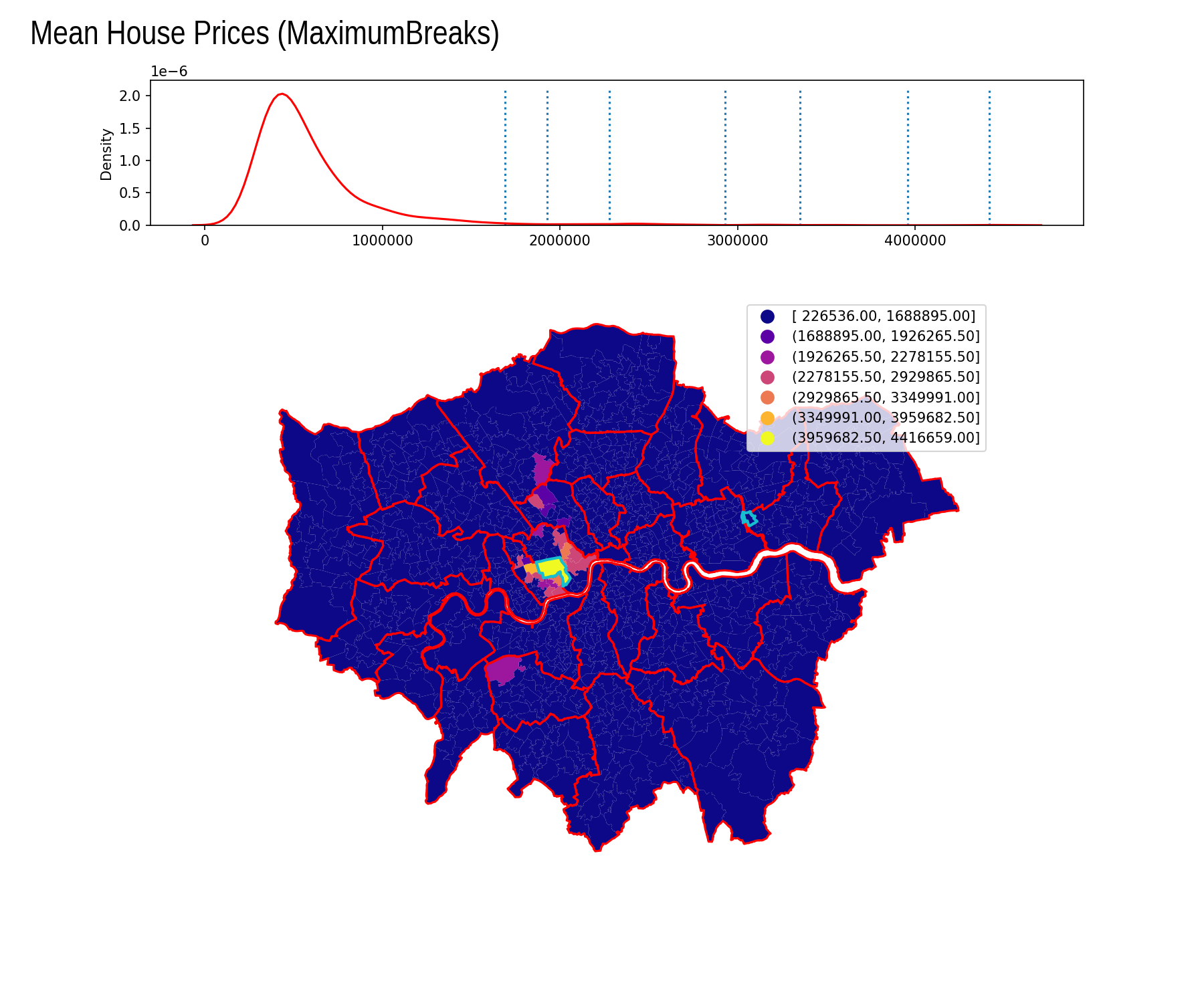
Maximum Breaks

Interval Count
[ 226536.00, 1688895.00] 961
(1688895.00, 1926265.50] 4
(1926265.50, 2278155.50] 5
(2278155.50, 2929865.50] 9
(2929865.50, 3349991.00] 2
(3349991.00, 3959682.50] 1
(3959682.50, 4416659.00] 1

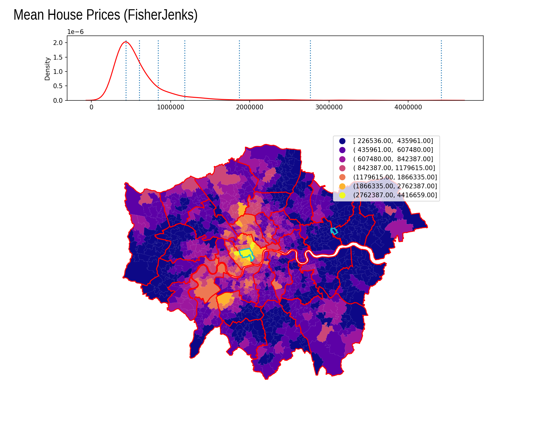
Fisher Jenks

Interval Count
[ 226536.00, 435961.00] 363
( 435961.00, 607480.00] 310
( 607480.00, 842387.00] 173
( 842387.00, 1179615.00] 80
(1179615.00, 1866335.00] 39
(1866335.00, 2762387.00] 14
(2762387.00, 4416659.00] 4

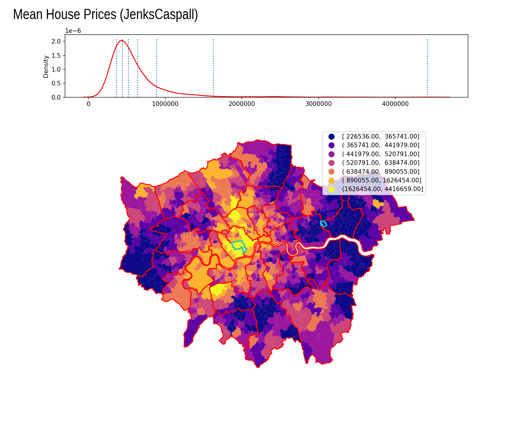
Jenks Caspall

Interval Count
[ 226536.00, 365741.00] 188
( 365741.00, 441979.00] 187
( 441979.00, 520791.00] 167
( 520791.00, 638474.00] 160
( 638474.00, 890055.00] 156
( 890055.00, 1626454.00] 103
(1626454.00, 4416659.00] 22

Summary

The choice of classification scheme should be data- and distribution-led. This is simply a demonstration of how different schemes can shape your understanding of the data.

Code (Useful Tips)

Setting up the classes:

kl = 7
cls = [mapclassify.BoxPlot, ...,  mapclassify.JenksCaspall]

Setting up the loop:

for cl in cls:
    try: 
        m = cl(ppd.Value, k=kl)
    except TypeError:
        m = cl(ppd.Value)
    
    f = plt.figure()
    gs = f.add_gridspec(nrows=2, ncols=1, height_ratios=[1,4])

    ax1 = f.add_subplot(gs[0,0])
    ...

    ax2 = f.add_subplot(gs[1,0])
    ...

Code (Useful Tips)

Setting up the distribution:

    ax1 = f.add_subplot(gs[0,0])
    sns.kdeplot(ppd.Value, ax=ax1, color='r')
    ax1.ticklabel_format(style='plain', axis='x') 

    y = ax1.get_ylim()[1]
    for b in m.bins:
        ax1.vlines(b, 0, y, linestyles='dotted')

Code (Useful Tips)

Adjusting the legend text:

def replace_legend_items(legend, mapping):
    for txt in legend.texts:
        for k,v in mapping.items():
            if txt.get_text() == str(k):
                txt.set_text(v)

Setting up the map:

    ax2 = f.add_subplot(gs[1,0])
    ppd.assign(cl=m.yb).plot(column='cl', k=len(m.bins), categorical=True, legend=True, ax=ax2)
    
    mapping = dict([(i,s) for i,s in enumerate(m.get_legend_classes())])
    ax2.set_axis_off()
    replace_legend_items(ax2.get_legend(), mapping)