Geopandas

Jon Reades

Pandas Learns about Maps

Geopandas

‘Geospatial Pandas’ provides a set of tools for working with geo-data in a pandas-like way. See: GeoPandas.org and Read the Docs.

PySAL

The Python Spatial Analysis Library provides an array of tools for performing spatial analysis. Now uses geo-pandas as default data structure. See: PySAL.org and Read the Docs.

Moving Pandas

A newer library that builds on Geopandas to offer movement analysis tools.

Basic Functionality

Reading & Writing

Supported file formats:

Type	Extension	Notes
Shape	.shp (etc.)	Maximum compatibility
GeoPackage	.gpkg	Good default choice
GeoJSON	.geojson	For web mapping
Zip	.zip	For use with Shapefiles
WKT	.txt	Plain-text & SQL
GeoParquet	.geoparquet	Good for large data sets & SQL

Additionally, it is possible to read only subsets of the data using row, column, geometry, and bbox filters.

Reading (Remote Files)

Again, depending on file size you may want to save these locally, but…

import geopandas as gpd
gpkg_src = 'https://bit.ly/2K4JcsB'
world = gpd.read_file(gpkg_src)
# The ';' suppresses matplotlib output
world.plot(facecolor='white', edgecolor='darkblue');

Writing (Local Files)

Write any OGR-supported vector drivers.

world.to_file('world.gpkg', driver='GPKG')
world.to_file('world.shp', driver='ESRI Shapefile')
world.to_file('world.geojson', driver='GeoJSON')

If you forget to specify the driver it writes shapefiles by default. This is mainly an issue if you try to write a GeoPackage or GeoJSON file but then end up writing a shapefile to a directory called world.gpkg!

Data Structures

GeoPandas does all this by adding just two new classes:

• GeoDataFrame
• GeoSeries

In principle, a GeoSeries can contain multiple geo-data types, but in practice you’ll want to be one of the following shapely classes:

1. Points / Multi-Points
2. Lines / Multi-Lines
3. Polygons / Multi-Polygons

Consider

Recall that we can ask if a particular object is an instance of any given class:

import pandas as pd
print(isinstance(world, str))
print(isinstance(world, pd.DataFrame))
print(isinstance(world, gpd.GeoDataFrame))

Prints: False, True, True.

import pandas as pd
print(isinstance(world.geometry, str))
print(isinstance(world.geometry, pd.Series))
print(isinstance(world.geometry, gpd.GeoSeries))

Also prints: False, True, True.

So converting from Pandas to GeoPandas works well because GeoPandas knows all about Pandas.

You can use a GeoDataFrame anywhere you’d use a DataFrame with no loss of functionality! Same for a GeoSeries, though in this case a GeoSeries cannot perform the same statistical operations.

Projections

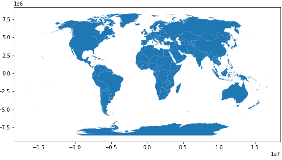
Depending on your data source, you may or may not have projection information attached to your GeoDataFrame:

print(world.crs)

outputs epsg:4326, but:

world.crs

outputs:

<Geographic 2D CRS: EPSG:4326>
Name: WGS 84
Axis Info [ellipsoidal]:
- Lat[north]: Geodetic latitude (degree)
- Lon[east]: Geodetic longitude (degree)
Area of Use:
- name: World
- bounds: (-180.0, -90.0, 180.0, 90.0)
Datum: World Geodetic System 1984
- Ellipsoid: WGS 84
- Prime Meridian: Greenwich

Finding Projections

You’ll have already covered this in GIS, but you can find nearly any EPSG you might need at epsg.io. By far the most commonly-used here are:

• EPSG:4326 for the World Geodetic System 84 used in GPS.
• EPSG:27700 for OSGB 1936/British National Grid used in the UK.

Note: recall that large territories (such as Canada, China and Russia) may well have multiple projections at the state of provincial level.

Reprojection

For data sets without projection information (i.e. often anything loaded from a shapefile) you must gdf.set_crs(<spec>). For all others you should gdf.to_crs(<spec>).

world2 = world.to_crs('ESRI:54030')
world2.plot();

Unlike a shapefile, you can have more than one geometry column, each with a different projection. However, only one will be plotted (the one named geometry or specified via set_geometry()).

The Spatial Index

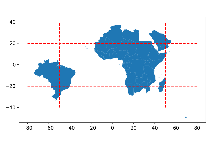
We can use GeoSeries’ spatial index directly to perform simple spatial queries:

import matplotlib.pyplot as plt
wslice = world.cx[-50:50, -20:20] # cx = coordinate index
ax = wslice.plot()
plt.axvline(-50, linestyle='--', color='red')
plt.axvline(50, linestyle='--', color='red')
plt.axhline(-20, linestyle='--', color='red')
plt.axhline(20, linestyle='--', color='red');

Attributes

A GeoSeries has attributes like any other Series, but also includes some spatially-specifc ones:

• area — if a polygon
• bounds — for each feature
• total_bounds — for each GeoSeries
• geom_type — if you don’t already know
• is_valid — if you need to test

Methods

Additional GeoSeries methods icnlude:

• distance() — returns Series measuring distances to some other feature (called as: <GeoSeries>.distance(<feature>))
• centroid — returns GeoSeries of strict centroids (called as: <GeoSeries>.centroid)
• representative_point() — returns GeoSeries of points within features
• to_crs() and plot(), which you’ve already seen.

Note that centroid is not called with parentheses. Technically it’s more like an attribute than a method.

Relationship Tests

Simple geographical tests:

• geom_almost_equals() — tries to deal with rounding issues when comparing two features.
• contains() — is shape contained within some other features.
• intersects() — does shape intersect some other features.

Point Data

Converting Non-Spatial Data 1

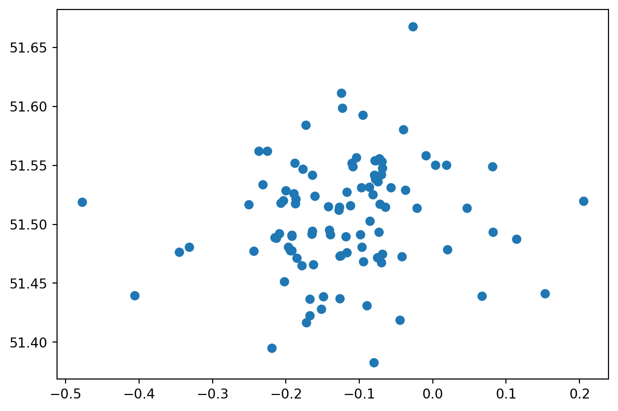
Lat/Long and Northing/Easting benefit from a helper function gpd.points_from_xy():

url = 'https://bit.ly/3I0XDrq'
df  = pd.read_csv(url)

gdf = gpd.GeoDataFrame(df, 
            geometry=gpd.points_from_xy(
                        df['longitude'], 
                        df['latitude'], 
                        crs='epsg:4326'
            )
      )
gdf.plot()

You can also use list comprehensions ([x for x in list]) and zip to combine two lists but then need to specify the CRS as a separate step!

CSV to Points in 3 Lines!

Notice that the default plot from a GeoDataFrame is… a map!

Converting Non-Spatial Data 2

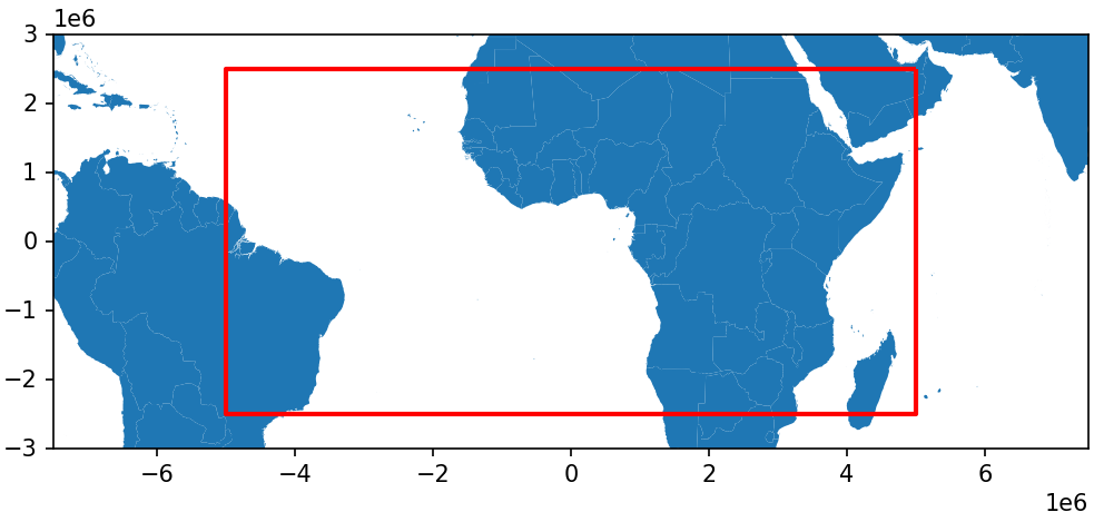
Other feature types need to be in some kind of regular format such as Well-Known Text (WKT), GeoJSON, or something readable as a Shapely geometry.

from shapely import wkt

# Notice coordinate pairs and last point is same as first one
bbox = 'POLYGON((5000000.0 2500000.0, 5000000.0 -2500000.0, -5000000.0 -2500000.0, -5000000.0 2500000.0, 5000000.0 2500000.0))'

# Create GeoPandas from dict just like Pandas
bgdf = gpd.GeoDataFrame({'id':[0], 'coordinates':bbox})

# Turn it into a geometry
bgdf['geometry'] = bgdf.coordinates.apply(wkt.loads)
bgdf = bgdf.set_crs('ESRI:54030')
bgdf.plot() # Not very interesting but...

These are more rarely used for our purposes but knowing that they exist is useful.

From Text to Bounding Box

scale = int(float('1e7'))
f,ax=plt.subplots(figsize=(8,4))
world2.plot(ax=ax)
bgdf.plot(ax=ax, color='none', edgecolor='r')
ax.set_xlim([-0.75*scale, +0.75*scale])
ax.set_ylim([-3*scale/10, +3*scale/10])

Resources

• I Hate Coordinate Systems
• GeoPandas on ReadTheDocs
• Dani’s GDS Course
• Dani’s Web Mapping Course