Exploratory Spatial Data Analysis
Jon Reades

For this one, you really need to read the docs.
Getting Spatial (with Boroughs)
import geopandas as gpd
url = 'https://bit.ly/3neINBV'
boros = gpd.read_file(url, driver='GPKG')
boros.plot(color='none', edgecolor='red');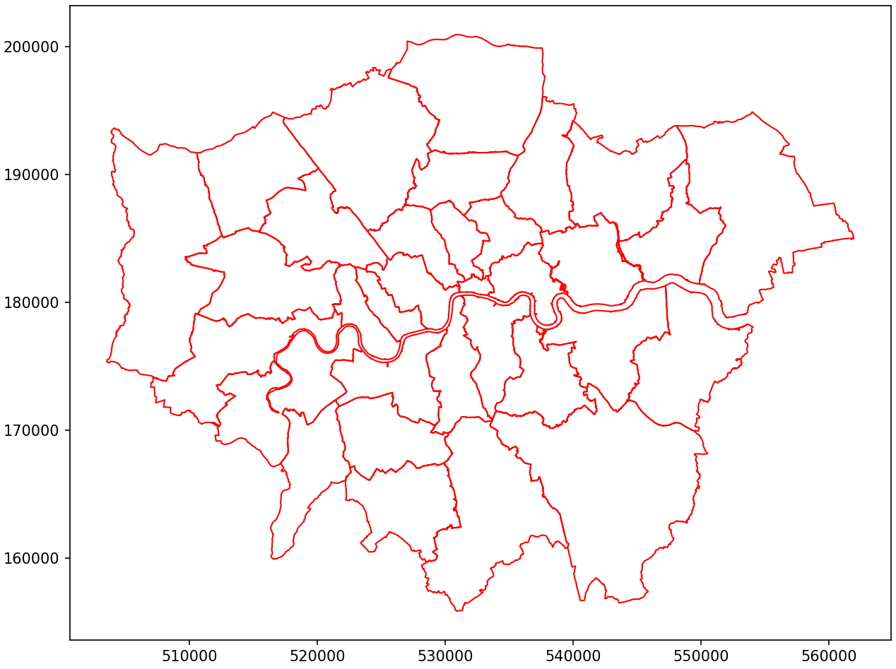
Convex Hull
boros['hulls'] = boros.geometry.convex_hull
boros = boros.set_geometry('hulls')
boros.plot(column='NAME', categorical=True, alpha=0.5);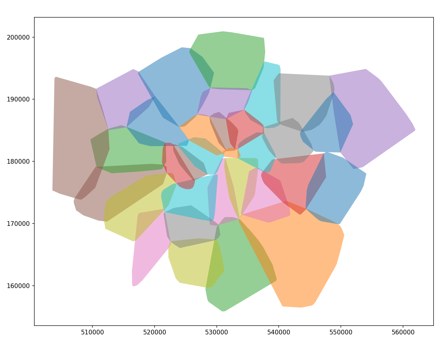
Dissolve
boros['region'] = 'London'
boros = boros.set_geometry('geometry') # Set back to original geom
ldn   = boros.dissolve(by='region')    # And dissolve to a single poly

f,ax = plt.subplots(figsize=(10,8))    # New plot
ldn.plot(ax=ax)                        # Add London layer to axis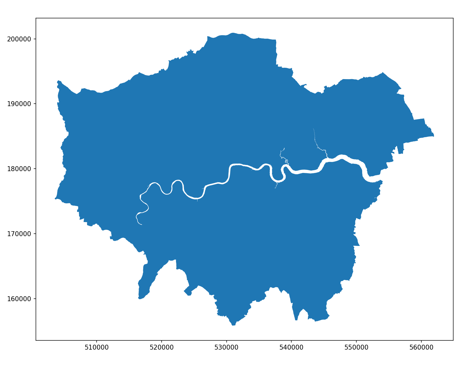
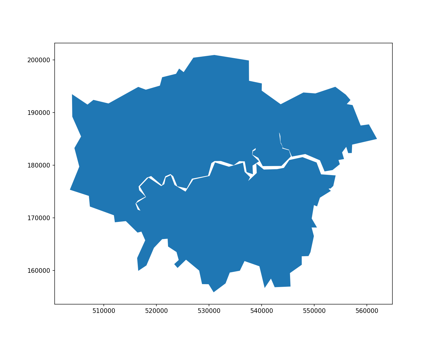
Simplify
Buffer
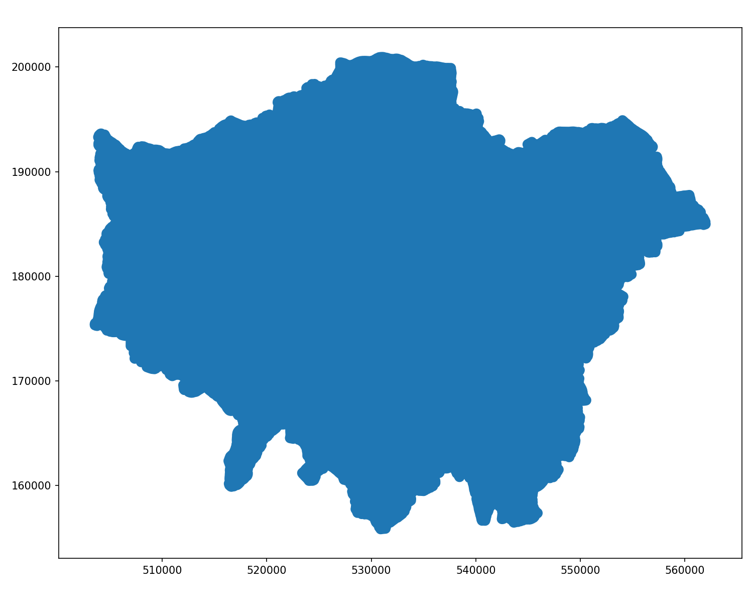
Buffer & Simplify
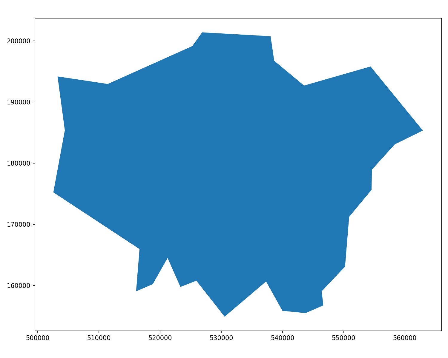
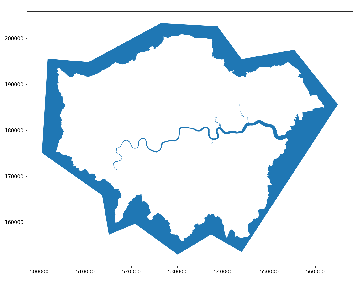
Difference
And some nice chaining…
Legendgrams
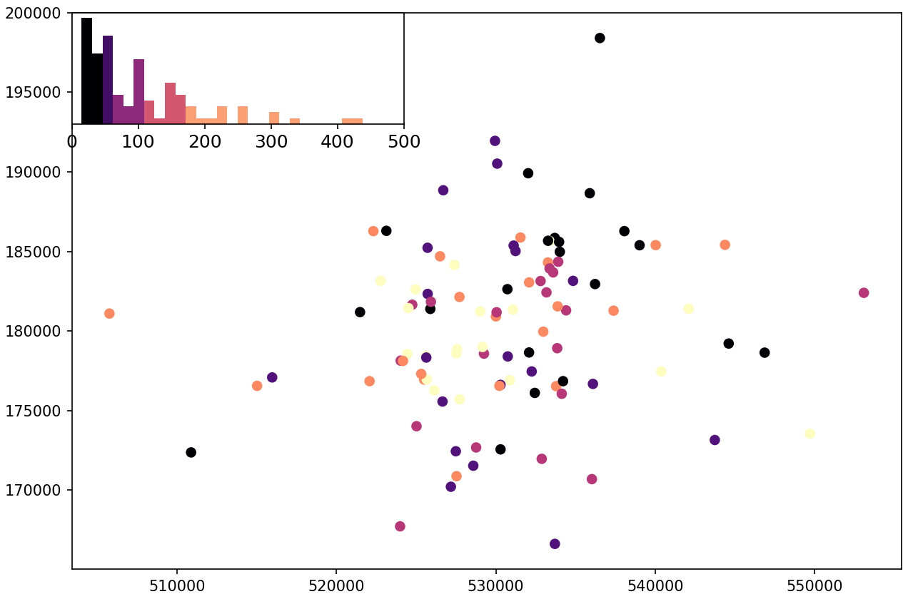
Implementing Legendgrams
import pysal as ps
# https://github.com/pysal/mapclassify
import mapclassify as mc
# https://jiffyclub.github.io/palettable/
import palettable.matplotlib as palmpl
from legendgram import legendgram

f,ax = plt.subplots(figsize=(10,8))
gdf.plot(column='price', scheme='Quantiles', cmap='magma', k=5, ax=ax)
q = mc.Quantiles(gdf.price.array, k=5)

# https://github.com/pysal/legendgram/blob/master/legendgram/legendgram.py
legendgram(f, ax,
               gdf.price, q.bins, pal=palmpl.Magma_5,
               legend_size=(.4,.2), # legend size in fractions of the axis
               loc = 'upper left', # mpl-style legend loc
               clip = (0,500), # clip range of the histogram
frameon=True)KNN Weights

Implementing KNN
from pysal.lib import weights
w = weights.KNN.from_dataframe(gdf, k=3)
gdf['w_price'] = weights.lag_spatial(w, gdf.price)
gdf[['name','price','w_price']].sample(5, random_state=42)| name | price | w_price | |
|---|---|---|---|
| 83 | Southfields Home | 85.0 | 263.0 |
| 53 | Flat in Islington, Central London | 55.0 | 190.0 |
| 70 | 3bedroom Family Home minutes from Kensington Tube | 221.0 | 470.0 |
| 453 | Bed, 20 min to Liverpool st, EAST LONDON | 110.0 | 186.0 |
| 44 | Avni Kensington Hotel | 430.0 | 821.0 |
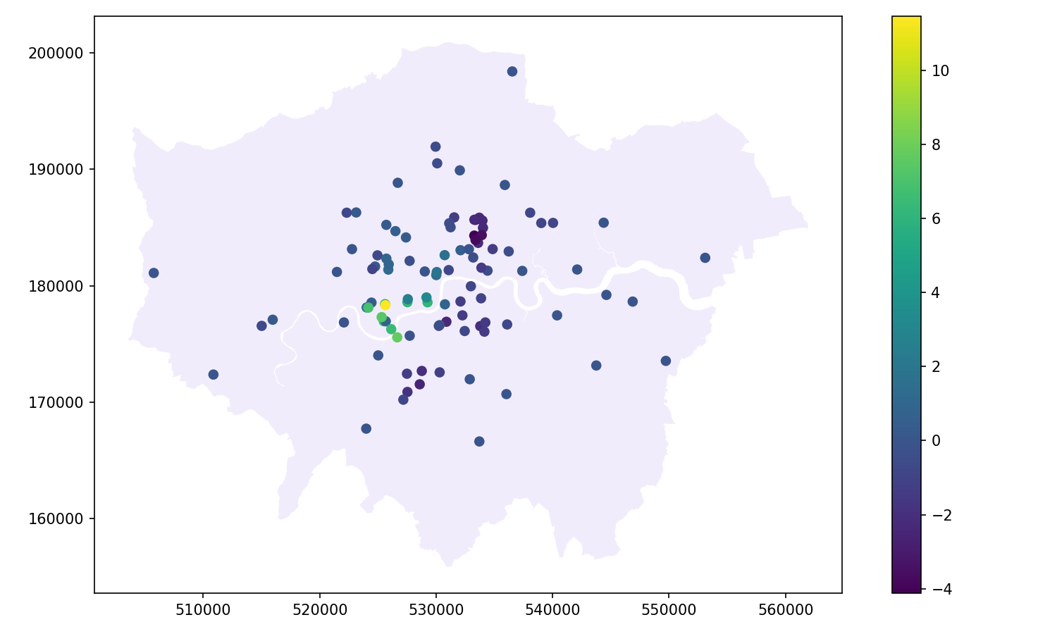
Spatial Lag of Distance Band
Implementing DB
w2 = weights.DistanceBand.from_dataframe(gdf, threshold=2000, alpha=-0.25)
gdf['price_std'] = (gdf.price - gdf.price.mean()) / gdf.price.std()
gdf['w_price_std'] = weights.lag_spatial(w2, gdf.price_std)
gdf[['name','price_std','w_price_std']].sample(5, random_state=42)| name | price_std | w_price_std | |
|---|---|---|---|
| 83 | Southfields Home | -0.27 | 0.00 |
| 53 | Flat in Islington, Central London | -0.51 | -0.58 |
| 70 | 3bedroom Family Home minutes from Kensington Tube | 0.83 | 0.46 |
| 453 | Bed, 20 min to Liverpool st, EAST LONDON | -0.07 | -0.82 |
| 44 | Avni Kensington Hotel | 2.52 | 3.25 |
Moran’s I
mi = esda.Moran(gdf['price'], w)
print(f"{mi.I:0.4f}")
print(f"{mi.p_sim:0.4f}")
moran_scatterplot(mi)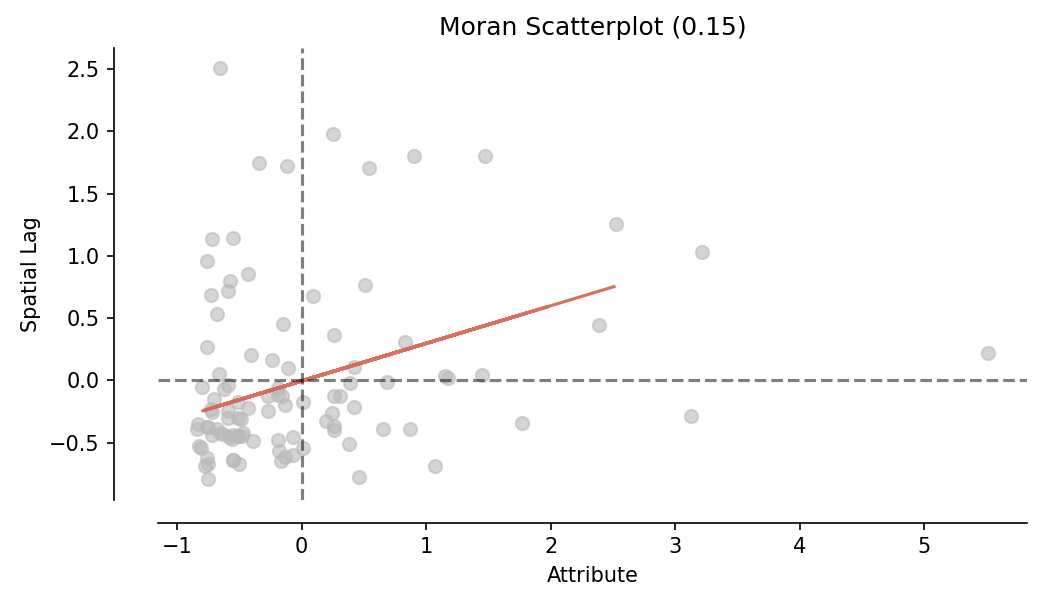
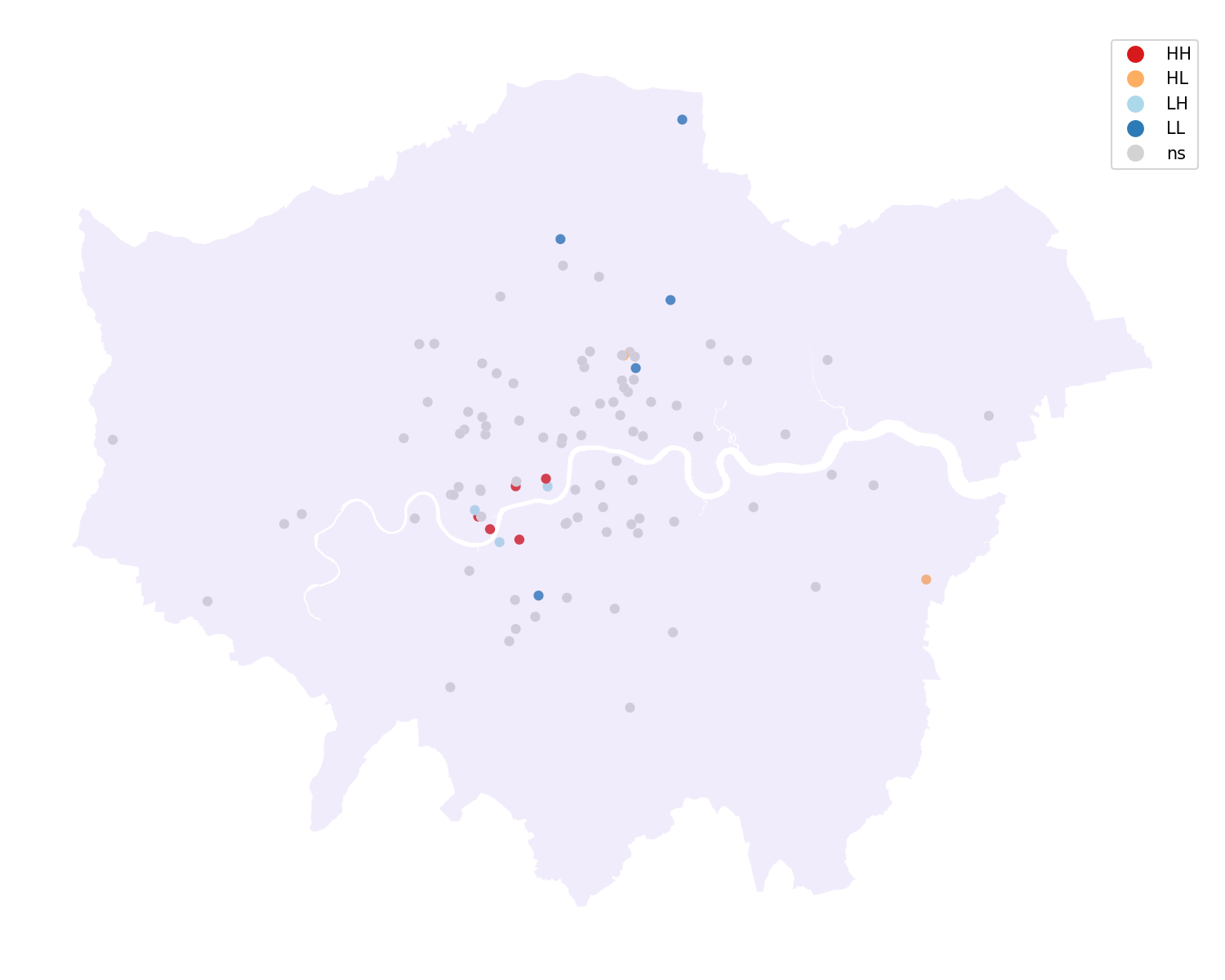
Local Moran’s I
Implementing Local Moran’s I
lisa = esda.Moran_Local(gdf.price, w)
# Break observations into significant or not
gdf['sig'] = lisa.p_sim < 0.05
# Store the quadrant they belong to
gdf['quad'] = lisa.q
gdf[['name','price','sig','quad']].sample(5, random_state=42)| name | price | sig | quad | |
|---|---|---|---|---|
| 83 | Southfields Home | 85.0 | False | 3 |
| 53 | Flat in Islington, Central London | 55.0 | False | 3 |
| 70 | 3bedroom Family Home minutes from Kensington Tube | 221.0 | False | 1 |
| 453 | Bed, 20 min to Liverpool st, EAST LONDON | 110.0 | False | 3 |
| 44 | Avni Kensington Hotel | 430.0 | False | 1 |
Full LISA

Resources
There’s so much more to find, but:
- Pandas Reference
- EDA with Pandas on Kaggle
- EDA Visualisation using Pandas
- Python EDA Analysis Tutorial
- Better EDA with Pandas Profiling [Requires module installation]
- Visualising Missing Data
- Choosing Map Colours

Exploratory Spatial Data Analysis • Jon Reades