Exploratory (Spatial) Data Analysis

Jon Reades - j.reades@ucl.ac.uk

1st October 2026

PySAL logo

For this one, you really need to read the docs.

Getting Spatial (with Boroughs)

import geopandas as gpd
url = 'https://bit.ly/3neINBV'
boros = gpd.read_file(url, driver='GPKG')
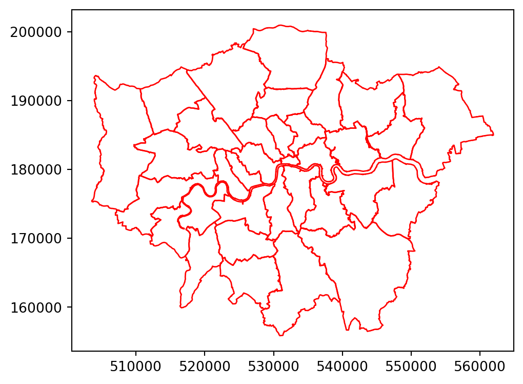
boros.plot(color='none', edgecolor='red', figsize=(8,4.5));

Plot of London boroughs

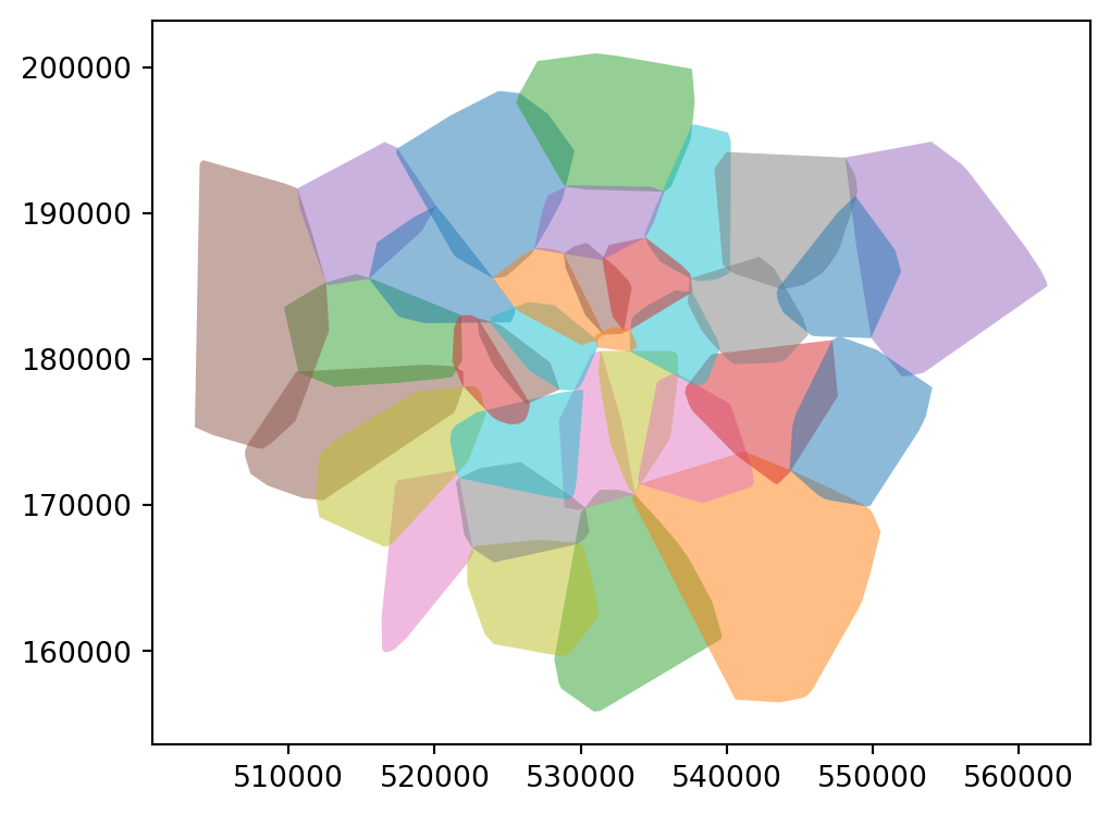
Convex Hull

boros['hulls'] = boros.geometry.convex_hull
boros.set_geometry('hulls').plot(column='NAME', categorical=True, alpha=0.5, figsize=(8,4.5));

Convex hull of London boroughs

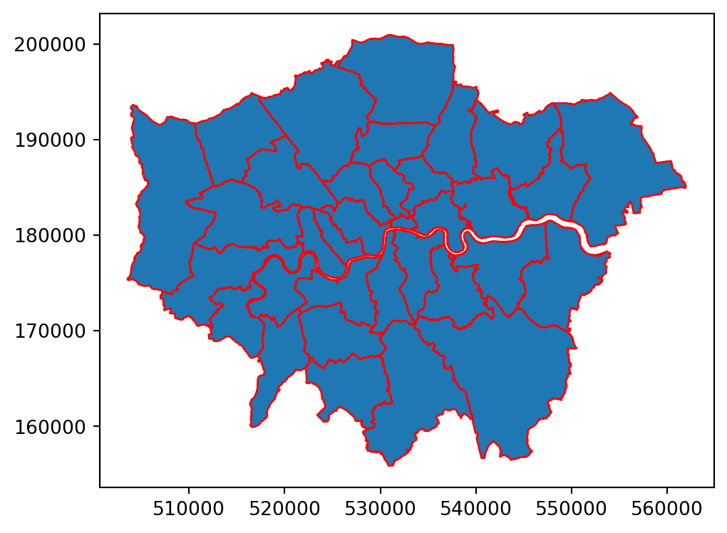
Dissolve

boros['region'] = 'London'
ldn   = boros.dissolve(by='region') 
ax = ldn.plot(figsize=(8,4.5)) 
boros.plot(ax=ax, color='none', edgecolor='red')

Dissolving London boroughs into the GLA region

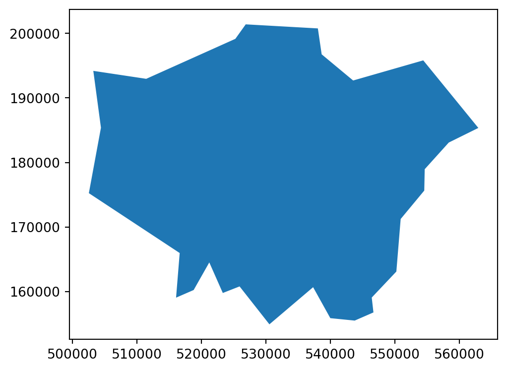
Buffer & Simplify

ldn.buffer(1000).simplify(1000).plot(figsize=(8,4.5))

Buffering the GLA area

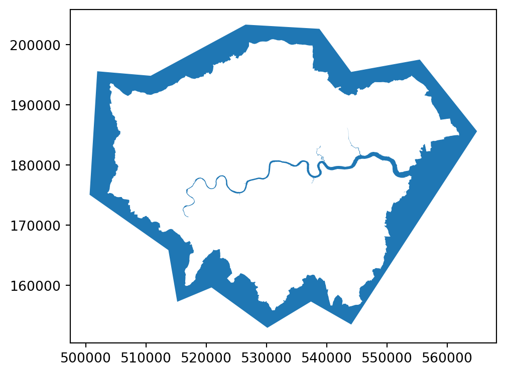
Difference

And some nice chaining…

ldn.buffer(3000).simplify(2500).difference(ldn.geometry).plot(figsize=(8,4.5))

Buffering, simplifying, and 'differencing' one geometry for its source

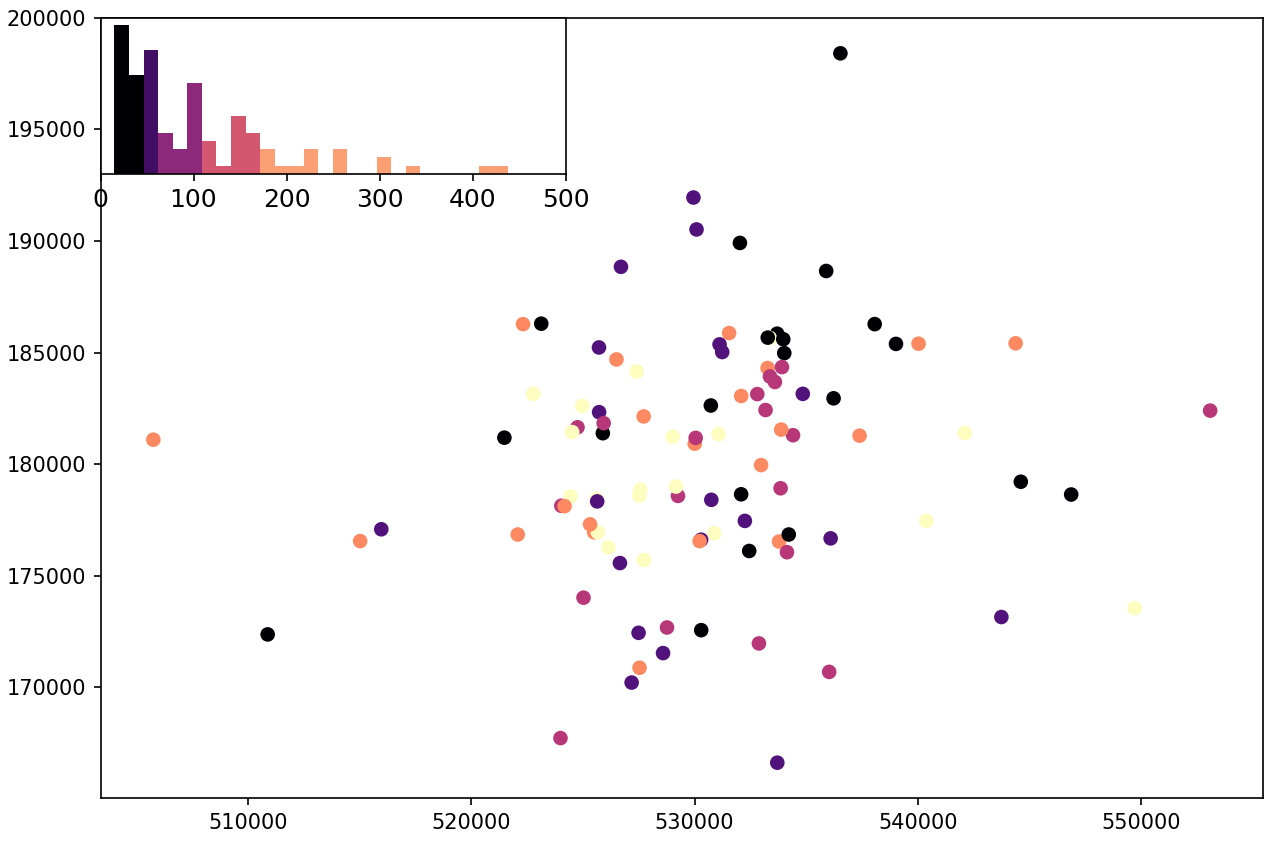
Legendgrams

Choropleth map with a legendgram: a histogram of the mapped values used as the legend

Implementing Legendgrams

import pysal as ps
# https://github.com/pysal/mapclassify
import mapclassify as mc
# https://jiffyclub.github.io/palettable/
import palettable.matplotlib as palmpl
from legendgram import legendgram

f,ax = plt.subplots(figsize=(10,8))
gdf.plot(column='price', scheme='Quantiles', cmap='magma', k=5, ax=ax)
q = mc.Quantiles(gdf.price.array, k=5)

# https://github.com/pysal/legendgram/blob/master/legendgram/legendgram.py
legendgram(f, ax, 
               gdf.price, q.bins, pal=palmpl.Magma_5,
               legend_size=(.4,.2), # legend size in fractions of the axis
               loc = 'upper left', # mpl-style legend loc
               clip = (0,500), # clip range of the histogram
               frameon=True)

KNN Weights

Map of Airbnb listings with lines connecting each listing to its k nearest neighbours

Implementing KNN

from pysal.lib import weights
w = weights.KNN.from_dataframe(gdf, k=3)
gdf['w_price'] = weights.lag_spatial(w, gdf.price)
gdf[['name','price','w_price']].sample(5, random_state=42)
name price w_price
83 Southfields Home 85.0 263.0
53 Flat in Islington, Central London 55.0 190.0
70 3bedroom Family Home minutes from Kensington Tube 221.0 470.0
453 Bed, 20 min to Liverpool st, EAST LONDON 110.0 186.0
44 Avni Kensington Hotel 430.0 821.0

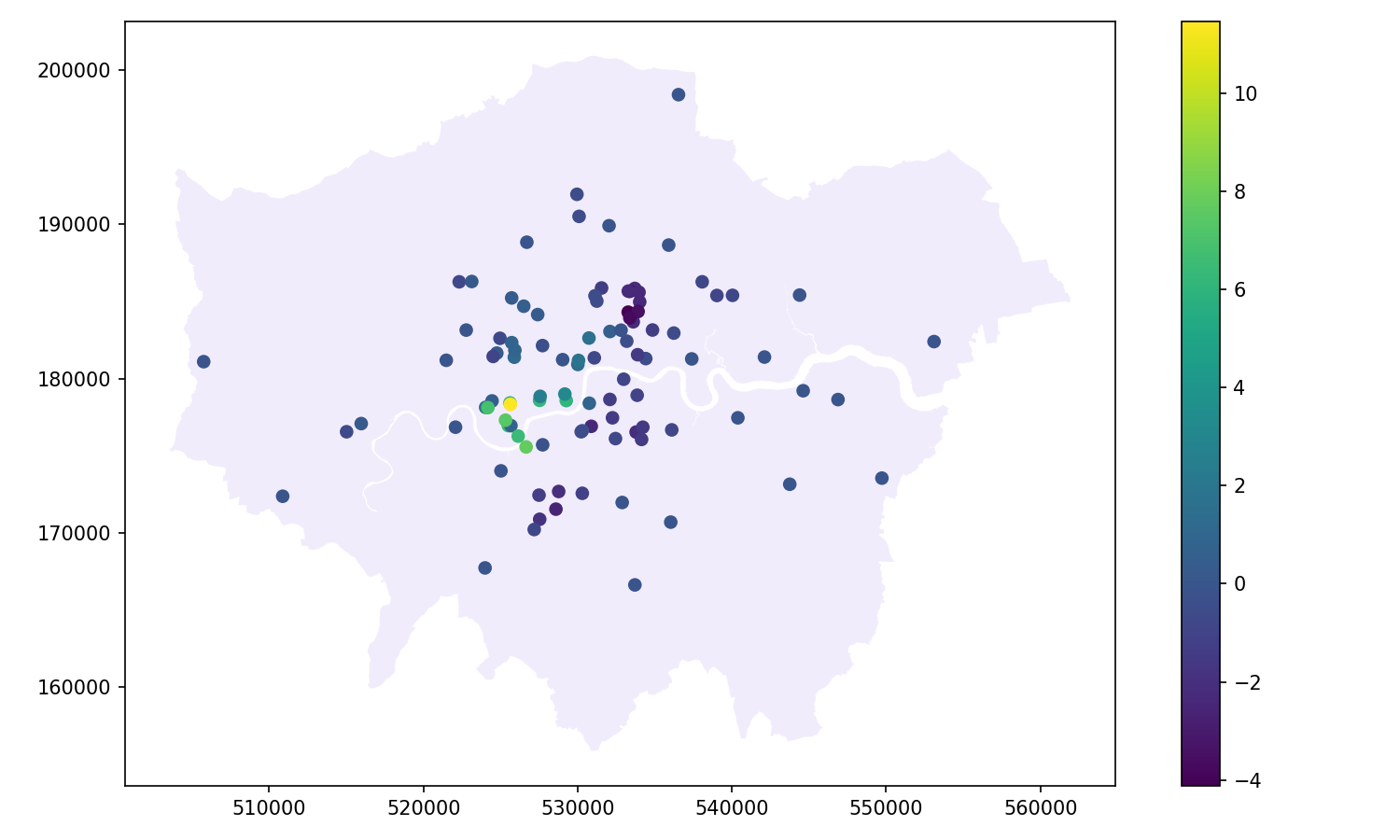
Spatial Lag of Distance Band

Map of the spatial lag of Airbnb prices calculated with distance-band weights

Implementing Lags

w2 = weights.DistanceBand.from_dataframe(gdf, threshold=2000, alpha=-0.25)
gdf['price_std'] = (gdf.price - gdf.price.mean()) / gdf.price.std()
gdf['w_price_std'] = weights.lag_spatial(w2, gdf.price_std)
gdf[['name','price_std','w_price_std']].sample(5, random_state=42)
name price_std w_price_std
83 Southfields Home -0.27 0.00
53 Flat in Islington, Central London -0.51 -0.58
70 3bedroom Family Home minutes from Kensington Tube 0.83 0.46
453 Bed, 20 min to Liverpool st, EAST LONDON -0.07 -0.82
44 Avni Kensington Hotel 2.52 3.25

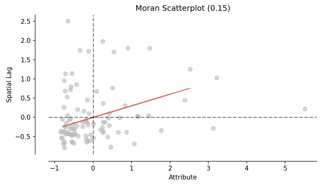
Moran’s I

mi = esda.Moran(gdf['price'], w)
print(f"{mi.I:0.4f}")
print(f"{mi.p_sim:0.4f}")
moran_scatterplot(mi)

Moran scatterplot of values against their spatial lag, whose slope is global Moran's I

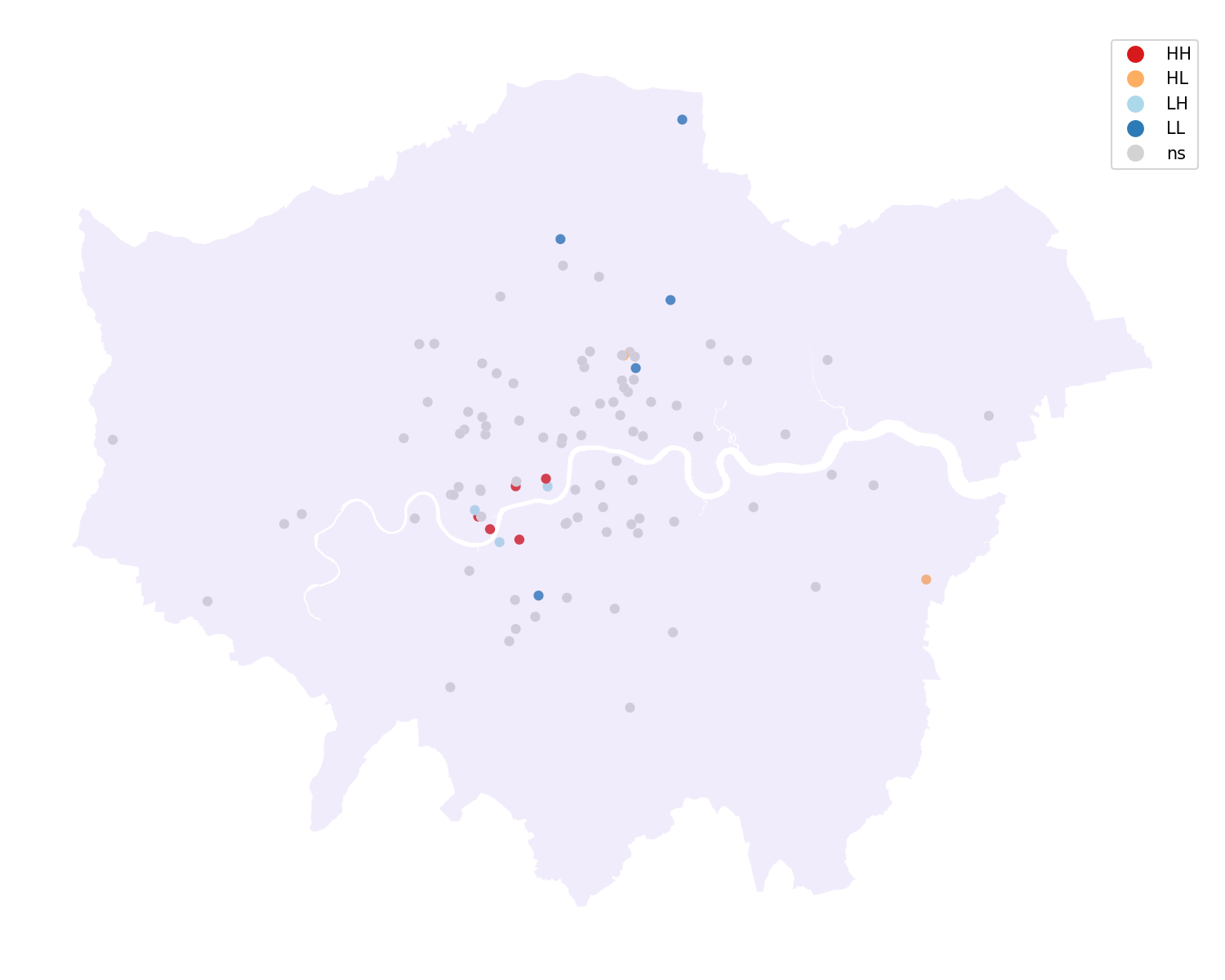
Local Moran’s I

Local Moran's I statistics plotted for each observation

Implementing Local Moran’s I

lisa = esda.Moran_Local(gdf.price, w)
# Break observations into significant or not
gdf['sig'] = lisa.p_sim < 0.05
# Store the quadrant they belong to
gdf['quad'] = lisa.q
gdf[['name','price','sig','quad']].sample(5, random_state=42)
name price sig quad
83 Southfields Home 85.0 False 3
53 Flat in Islington, Central London 55.0 False 3
70 3bedroom Family Home minutes from Kensington Tube 221.0 False 1
453 Bed, 20 min to Liverpool st, EAST LONDON 110.0 False 3
44 Avni Kensington Hotel 430.0 False 1

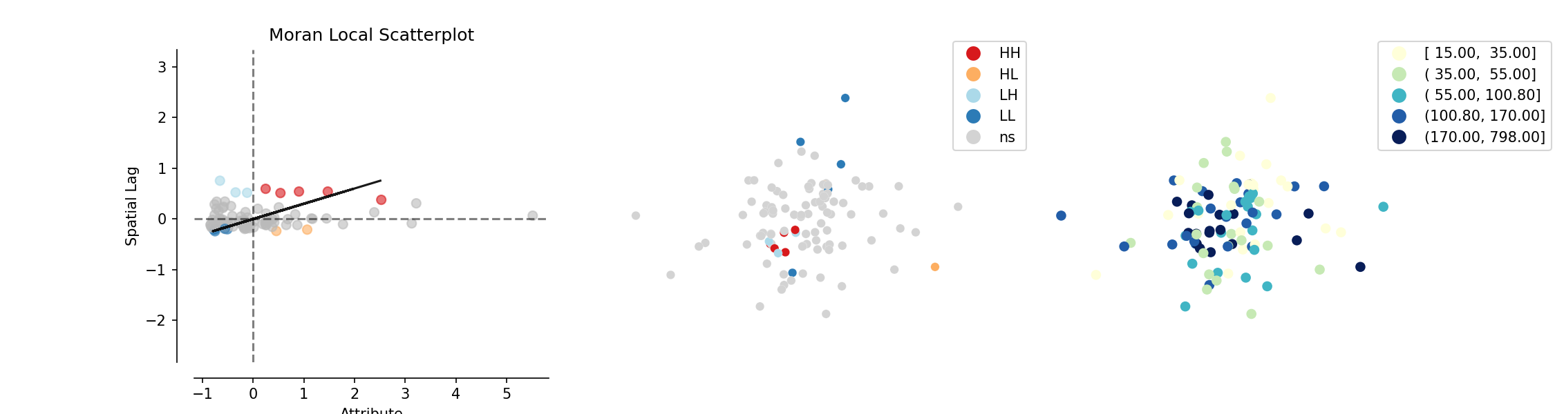
Full LISA

plot_local_autocorrelation(lisa, gdf, 'price')

LISA panel: a Moran scatterplot, a cluster map of hot and cold spots, and a choropleth of Airbnb prices

Additional Resources

There’s so much more to find, but:

Thank You

References