Analysing Text

Jon Reades - j.reades@ucl.ac.uk

1st October 2026

Dummy Values?

What’s wrong with this approach?¹

	Topic Text	Topic Number
Article 1	News	1
Article 2	Culture	2
Article 3	Politics	3
Article 4	Entertainment	4

What’s the problem with this approach when you’re thinking about the topics in a document? You either have to assign each document to one, and only one, topic, or you need a lot of dummies.

1. If you can spot the problem right away, congratulations! I didn’t see it for a few years because everyone else thought it was too obvious to explain!

Dummy Variables Columns!

	News	Culture	Politics
Article 1	1	0	0
Article 2	0	1	0
Article 3	0	0	1
Article 4	0	0	0

One-Hot Encoders

	News	Culture	Politics	Entertainment
Article 1	1	0	0	0
Article 2	0	1	0	0
Article 3	0	0	1	0
Article 4	0	0	0	1

So the big difference is One Hot == \(n\) variables, Dummy == \(n-1\).

Definitely some ‘gotchas’ in deployment: one-hot models shouldn’t have an intercept unless you apply a ‘ridge shrinkage penalty’. Standardisation affects whether or not an intercept is needed.

The ‘Bag of Words’

Just like a one-hot (binarised approach) on preceding slide but now we count occurences:

Document	UK	Top	Pop	Coronavirus
News item	4	2	0	6
Culture item	0	4	7	0
Politics item	3	0	0	3
Entertainment item	3	4	8	1

BoW in Practice

Enter, stage left, scikit-learn:

from sklearn.feature_extraction.text import CountVectorizer
vectorizer = CountVectorizer()

# Non-reusable transformer
vectors = vectorizer.fit_transform(texts)

# Reusable transformer
vectorizer.fit(texts)
vectors1 = vectorizer.transform(texts1)
vectors2 = vectorizer.transform(texts2)

print(f'Vocabulary: {vectorizer.vocabulary_}')
print(f'All vectors: {vectors.toarray()}')

TF/IDF

Builds on Count Vectorisation by normalising the document frequency measure by the overall corpus frequency. Common words receive a large penalty:

\[ W(t,d) = TF(t,d) / log(N/DF_{t}) \]

For example:

• If the term ‘cat’ appears 3 times in a document of 100 words then Term Frequency given by: \(TF(t,d)=3/100\), and
• If there are 10,000 documents and cat appears in 1,000 documents then Normalised Document Frequency given by: \(N/DF_{t}=10000/1000\) so the Inverse Document Frequency is \(log(10)=1\),
• So IDF=1 and TF/IDF=0.03.

TF/IDF in Practice

from sklearn.feature_extraction.text import TfidfVectorizer
vectorizer = TfidfVectorizer()

# Non-reusable form:
vectors=vectorizer.fit_transform(texts)

# Reusable form:
vectorizer.fit(texts)
vectors = vectorizer.transform(texts)

print(f'Vocabulary: {vectorizer.vocabulary_}')
print(f'Full vector: {vectors.toarray()}')

What do you notice about how this code differs from the CountVectorizer?

Term Co-Occurence Matrix (TCM)

Three input texts with a distance weighting (\(d/2\), where \(d<3\)):

• the cat sat on the mat
• the cat sat on the fluffy mat
• the fluffy ginger cat sat on the mat

	fluffy	mat	ginger	sat	on	cat	the
fluffy		1	1		0.5	0.5	2.0
mat					0.5		1.5
ginger				0.5	0.5	1.0	1.5
sat					3.0	3.0	2.5
on						1.5	3.0
cat							2.0
the

How Big is a TCM?

The problem:

• A corpus with 10,000 words has a TCM of size \(10,000^{2}\) (100,000,000)
• A corpus with 50,000 words has a TCM of size \(50,000^{2}\) (2,500,000,000)

Cleaning is necessary, but it’s not sufficient to create a tractable TCM on a large corpus.

Although usually used in the context of clustering, there’s also a curse of dimensionality here!

Enter Embeddings

Typically, some kind of 2 or 3-layer neural network that ‘learns’ how to embed the TCM into a lower-dimension representation: from \(m \times m\) to \(m \times n, n << m\).

Similar to PCA in terms of what we’re trying to achieve, but the process is utterly different.

Many different approaches, but GloVe (Stanford), word2vec (Google), fastText (Facebook), and ELMo (Allen) or BERT (Google) are probably the best-known.

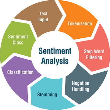
Sentiment Analysis

Requires us to deal in great detail with bi- and tri-grams because negation and sarcasm are hard. Also tends to require training/labelled data.

Source.

Clustering

Cluster	Geography	Earth Science	History	Computer Science	Total
1	126	310	104	11,018	11,558
2	252	10,673	528	126	11,579
3	803	485	6,730	135	8,153
4	100	109	6,389	28	6,626
Total	1,281	11,577	13,751	11,307	37,916

Topic Modelling

Learning associations of words (or images or many other things) to hidden ‘topics’ that generate them:

Word Clouds

Additional Resources

• One-Hot vs Dummy Encoding
• Categorical encoding using Label-Encoding and One-Hot-Encoder
• Count Vectorization with scikit-learn
• Corpus Analysis with Spacy
• The TF*IDF Algorithm Explained
• How to Use TfidfTransformer and TfidfVectorizer
• SciKit Learn Feature Extraction
• Your Guide to LDA
• Machine Learning — Latent Dirichlet Allocation LDA
• A Beginner’s Guide to Latent Dirichlet Allocation(LDA)
• Analyzing Documents with TF-IDF

Basically any of the lessons on The Programming Historian.

Additional Resources

• Introduction to Word Embeddings
• The Current Best of Universal Word Embeddings and Sentence Embeddings
• Using GloVe Embeddings
• Working with Facebook’s FastText Library
• Word2Vec and FastText Word Embedding with Gensim
• Sentence Embeddings. Fast, please!

• PlasticityAI Embedding Models
• Clustering text documents using k-means
• Topic extraction with Non-negative Matrix Factorization and LDA
• Topic Modeling with LSA, pLSA, LDA, NMF, BERTopic, Top2Vec: a Comparison

Thank You

References