| SensorID | Latitude | Longitude | |
|---|---|---|---|
| 0 | 1 | 51.5070 | -0.1347 |
| 1 | 2 | 51.5071 | -0.0042 |
| 2 | 3 | 51.5074 | -0.1223 |
| 3 | 4 | 51.5073 | -0.1122 |
| 4 | 5 | 51.5073 | 0.1589 |
Linking (Spatial) Data
Jon Reades - j.reades@ucl.ac.uk
1st October 2025
> Spatial data connected in more complex ways unlocking even more applications, but at a cost!
Non-Spatial Linkages can be Spatial
Data Set 1
Data Set 2
Going Spatial
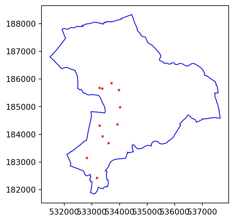
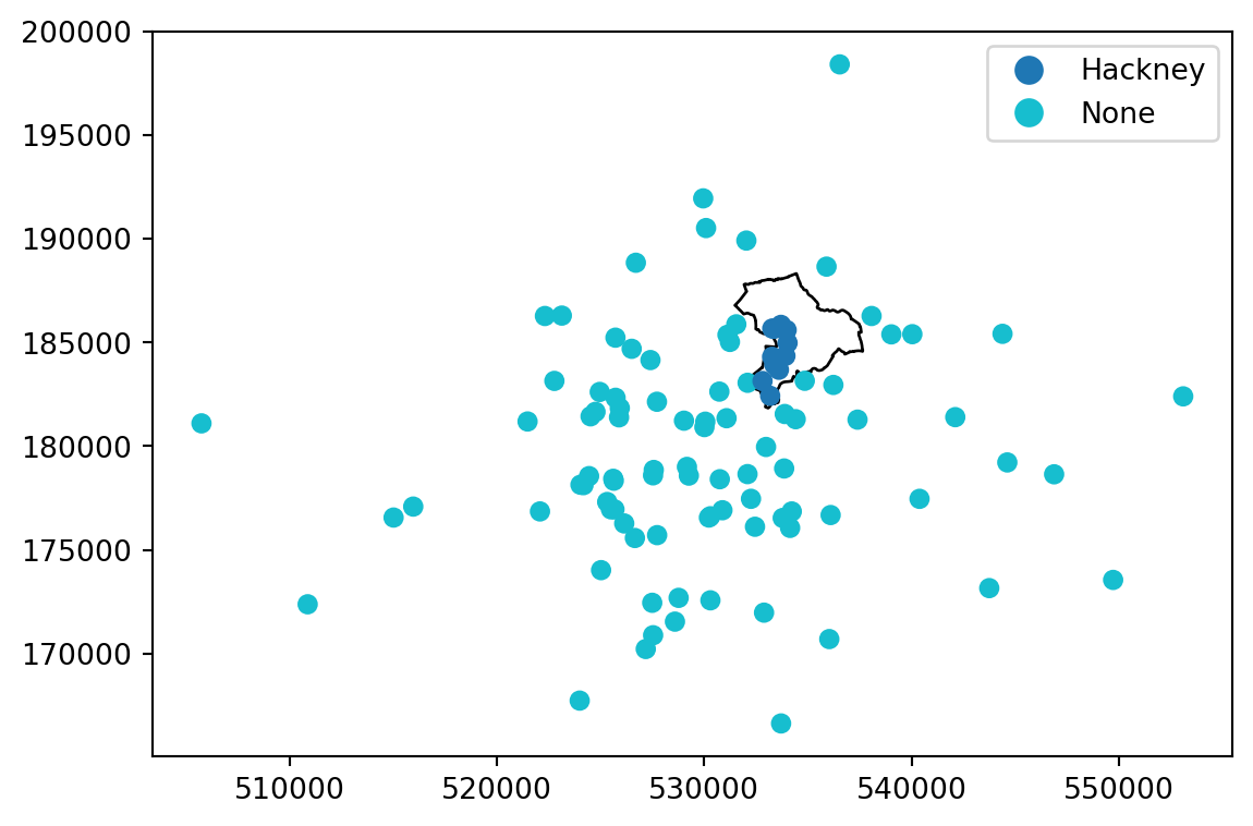
A Spatial Join
Sjoin adds an predicate ('intersects','contains','within'):
Combining Operators & How
Changing how to left, right, or inner changes the join’s behaviour:
Merging Data
These merge operators apply where a is the left set of features (in a GeoSeries or GeoDataFrame) and b is the right set:
- Contains: Returns
Trueif no points of b lie outside of a and at least one point of b lies inside a. - Within: Returns
Trueif a’s boundary and interior intersect only with the interior of b (not its boundary or exterior). - Intersects: Returns
Trueif the boundary or interior of a intersects in any way with those of b.
All binary predicates are supported by features of GeoPandas, though only these three options are available in sjoin directly.
Additional Spatial Operations
These operators apply to the GeoSeries where a is a GeoSeries and b is one or more spatial features:
- Contains / Covers: Returns a
Seriesofdtype('bool')with valueTruefor each geometry inathat containsb. These are different. - Crosses: An object is said to cross other if its interior intersects the interior of the other but does not contain it, and the dimension of the intersection is less than the dimension of the one or the other.
- Touches: Returns a
Seriesindicating which elements ofatouch a point onb. - Distance: Returns a
Seriescontaining the distance from allato someb. - Disjoint: Returns a
Seriesindicating which elements ofado not intersect with anyb. - Geom Equals / Geom Almost Equals: strict and loose tests of equality between
aandbin terms of their geometry. - Buffer, Simplify, Centroid, Representative Point: common transformations.
- Rotate, Scale, Affine Transform, Skew, Translate: less common transformations.
- Unary Union: aggregation of all the geometries in
a
RTM
In particular, “contains” (and its converse “within”) has an aspect of its definition which may produce unexpected behaviour. This quirk can be expressed as “Polygons do not contain their boundary”. More precisely, the definition of contains is: Geometry A contains Geometry B iff no points of B lie in the exterior of A, and at least one point of the interior of B lies in the interior of A That last clause causes the trap – because of it, a LineString which is completely contained in the boundary of a Polygon is not considered to be contained in that Polygon! This behaviour could easily trip up someone who is simply trying to find all LineStrings which have no points outside a given Polygon. In fact, this is probably the most common usage of contains. For this reason it’s useful to define another predicate called covers, which has the intuitively expected semantics: Geometry A covers Geometry B iff no points of B lie in the exterior of A
Set Operations with Overlay
It is also possible to apply GIS-type ‘overlay’ operations:
These operations return indexes for gdf1 and gdf2 (either could be a NaN) together with a geometry and (usually?) columns from both data frames:
The set of operations includes: union, intersection, difference, symmetric_difference, and identity.
Making a Plan…
Think it Through
As your data grows in volume, the consequences of choosing the ‘wrong’ approach become more severe. Making a plan of attack becomes essential and it boils down to the following:
- Spatial joins are hard
- Non-spatial joins are easy
- Key-/Index-based joins are easiest
- Addition conditions to joins makes them harder.
So, when you have multiple joins…
- Do the easy ones first (they will run quickly on large data sets).
- Do the hard ones last (they will benefit most from the filtering process).
What’s the ‘Right’ Order?
Q. Find me a nearby family-style Italian restaurant…
A. Here’s how I’d do this:
- City = New York (probably a key)
- Cuisine = Italian (probably a key)
- Style = Family (probably an enumeration/free text)
- Location = Within Distance of X from Request (probably a buffered spatial query)
- Style = Family (probably an enumeration/free text)
- Cuisine = Italian (probably a key)
Mis-matched Scales
Keep in mind:
With complex geometries and mis-matched scales, converting the smaller geometry to centroids or representative points can speed things up a lot (within, contains, etc. become much simpler).
And that:
With large data sets, rasterising the smaller and more ‘abundant’ geometry can speed things up a lot.
> Long term: if you continue to work with large spatial data sets you’ll need to look into web services and spatial databases.
Web Services
| Acronym | Means | Does |
|---|---|---|
| WMS | Web Map Service | Transfers map images within an area specified by bounding box; vector formats possible, but rarely used. |
| WFS | Web Feature Service | Allows interaction with features; so not about rendering maps directly, more about manipulation. |
| WCS | Web Coverage Service | Transfers data about objects covering a geographical area. |
| OWS | Open Web Services | Seems to be used by QGIS to serve data from a PC or server. |
Spatial Databases
There are many flavours:
- Oracle: good enterprise support; reasonably feature-rich, but £££ for commercial use.
- MySQL: free, unless you want dedicated support; was feature-poor (though this looks to have changed with MySQL8); heavyweight.
- PostgreSQL: free, unless you want dedicated support; standards-setting/compliant; heavyweight (requires PostGIS).
- Microsoft Access: um, no.
- SpatiaLite: free; standards-setting/compliant; lightweight
- GeoParquet+DuckDB: not as full-featured as Postgres, but evolving quickly and much simpler to configure.
Generally:
- Ad-hoc, modestly-sized, highly portable == SpatiaLite
- Permanent, large, weakly portable == Postgres+PostGIS


