Hello, QGIS!
QGIS is constantly evolving, so from time to time they make changes that impact the UI (User Interface). Don’t stress if what you’re seeing in QGIS on your monitor differs slightly from the screenshots here: take a minute to see if things are similar but just look a bit different, look around to see if things have just moved, and use Google if you need to.
1 Getting Started
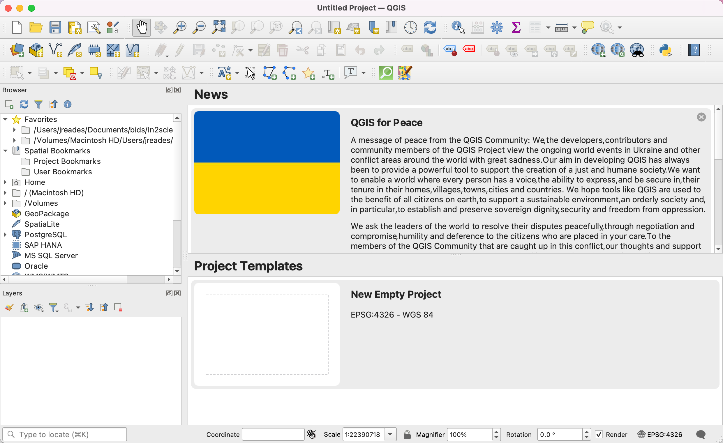
QGIS can be found under the Raspberry Pi menu (top-left) and then in Education. Start QGIS and you’ll get a welcome page showing previously created projects (if any) and some general information about QGIS. Next, create a new, empty document by clicking on the… wait for it… `New Empty Document’ area visible on the Welcome Page or on the ‘blank’ document icon at the top-left of the screenshot below.
2 Adding OSM Data
OSM stands for ‘Open Street Map’ and it’s the largest open data set in the world – companies like Apple and Uber rely on OSM (and contribute data to it) so that they aren’t dependent on Google!
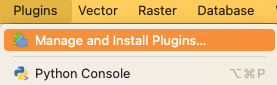
What if you don’t see Quick Map Services under the Web menu? Don’t panic! This service is a plugin and you can you can install it by clicking on the plugin menu item, selecting ’’
2.1 Add OSM Map Layer
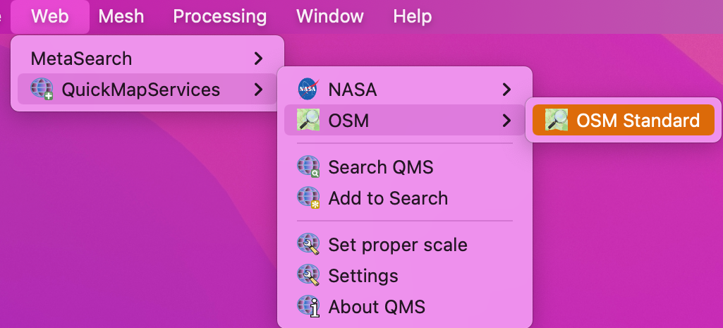
Under the Web menu item at the top of your screen is a QuickMapServices option:
- Under
Webin the main application window… - Pick
QuickMapServices - Pick
OSM(Open Street Map) - Pick
OSM Standard
2.2 Find Brixton
Now zoom in on London using the magnifying glass (with the +) as below:
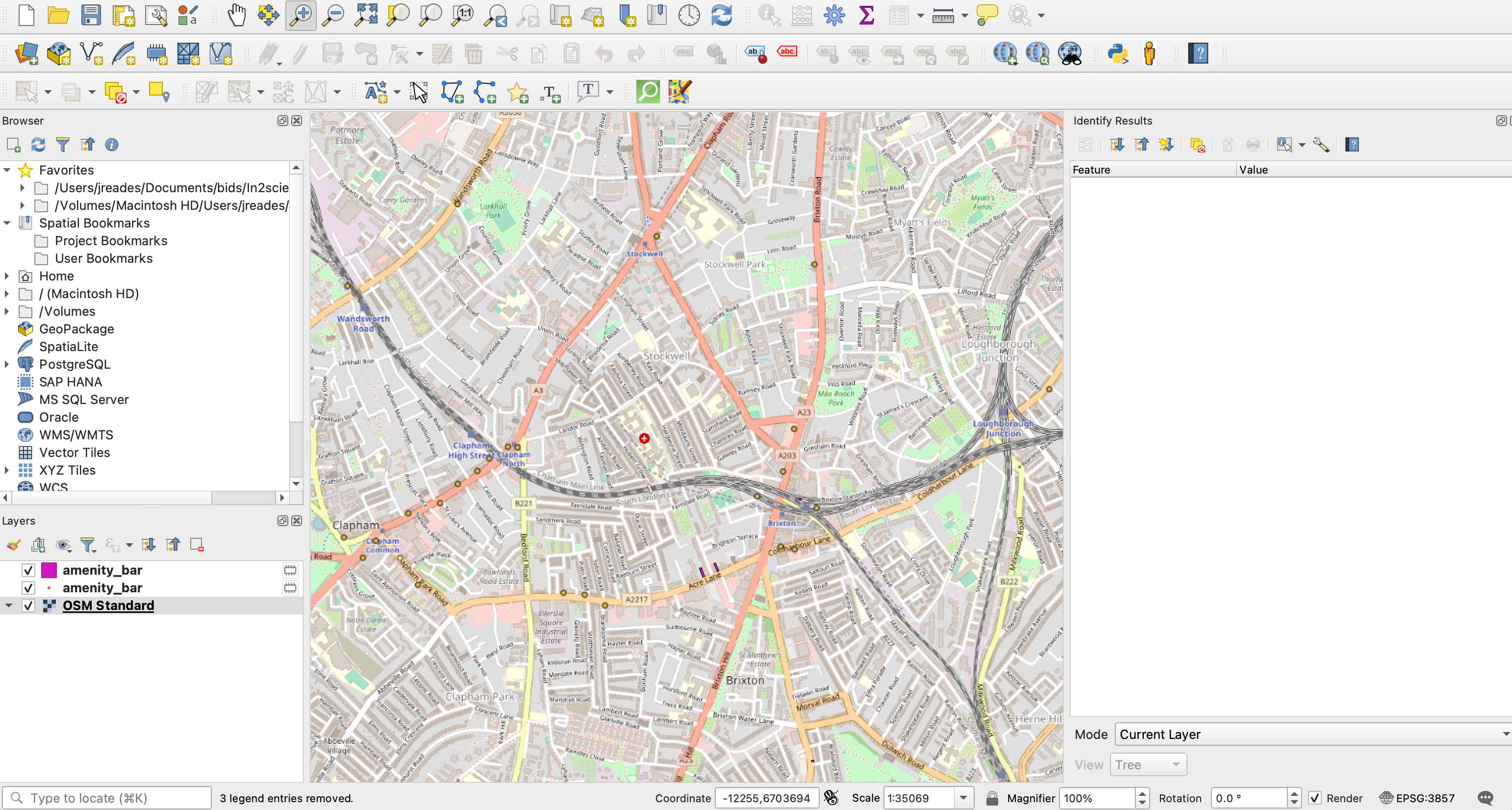
Panning (keeping the same zoom level but noving the map) is done using the Hand icon or by pressing the space bar and dragging the mouse. If you leave the mouse hovering over a button you will get some simple help to tell you what the button does. See if you can get Brixton in the centre of the map!

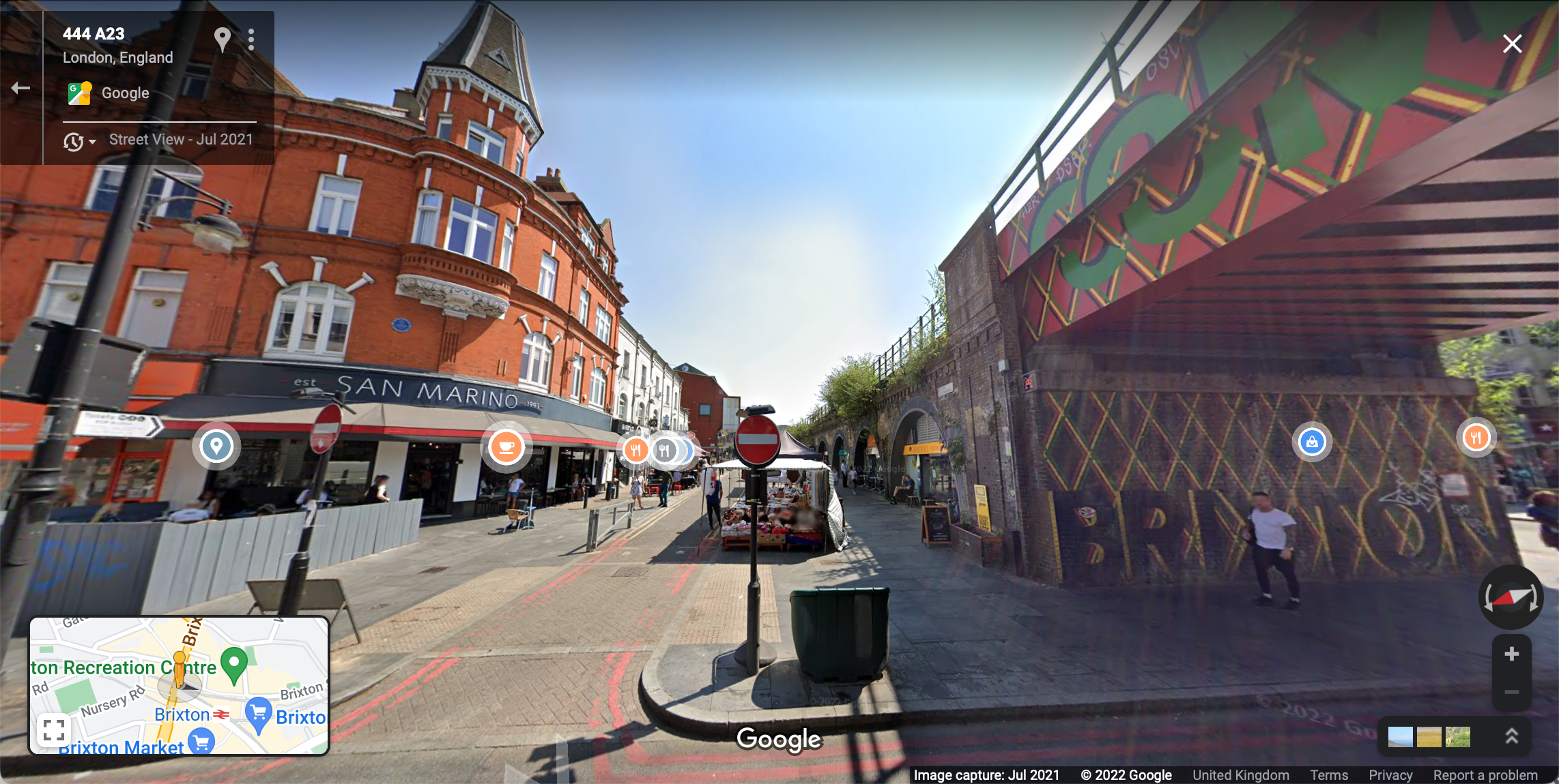
2.3 Check Out Street View
If you click on the Google Street View icon (![]() ) and then click+drag anywhere on the map you will open Google Street View in your web browser showing the view from that point in the direction selected.
) and then click+drag anywhere on the map you will open Google Street View in your web browser showing the view from that point in the direction selected.
Google Street View is also a plugin that you can install yourself. Many bits of useful functionality are provided by others: that’s the open source benefit… occassionally a cost when a useful plugin is abandoned.
2.4 Add Some ‘Real’ Data
Under the Vector menu you’ll see a QuickOSM option, and then a second QuickOSM menu item. select this. This will open a new popup menu.
We are now going to build a query, meaning that we’ll be asking OpenStreetMap’s servers to find us locations fitting a particular description/having a particular tag. There are many tags and many choices, so a good way to find out what you want is to Google OSM wiki <x> where <x> is whatever you’re looking for (e.g. yoga studios, bars, etc.).
London has a lot of data, so you must change the In drop-down to Canvas Extent and ensure you’re fairly zoomed-in on Brixton if you don’t want to be waiting a very long time for data.
As a first go, your query could look like this one for ‘local bars’:
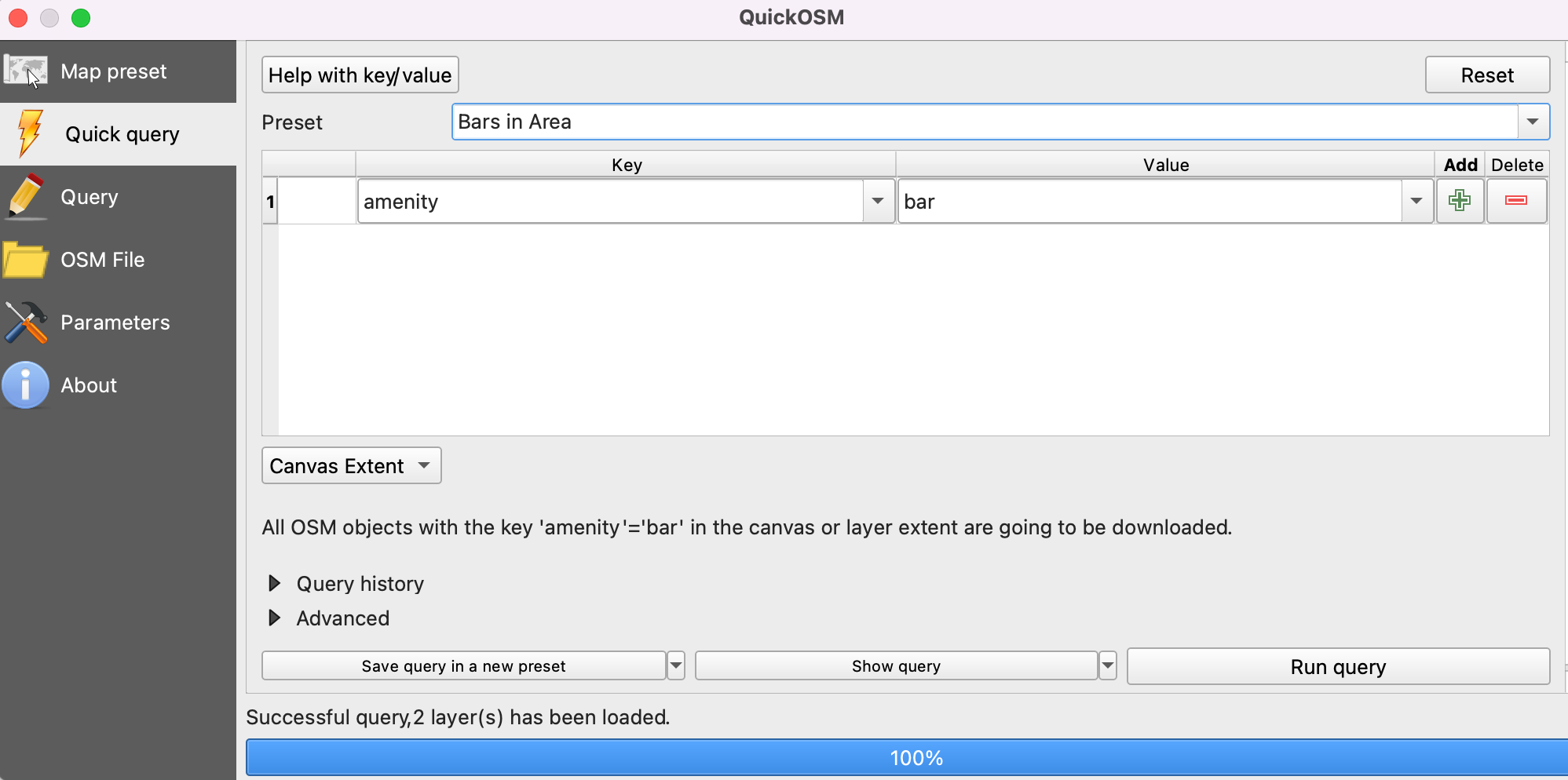
Depending on how far you were zoomed in when you created this query, after clicking Run Query you might get an answer nearly instantly or have to wait up to a couple of minutes! When the query completes you should see that two new layers have appeared in the lower left-hand corner of the QGIS app:
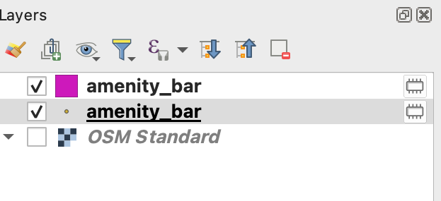
If you’re having trouble seeing the bars that you’ve added, try turning off the OSM Standard layer by clicking the tic-box next to its name!
2.5 More Information Please!
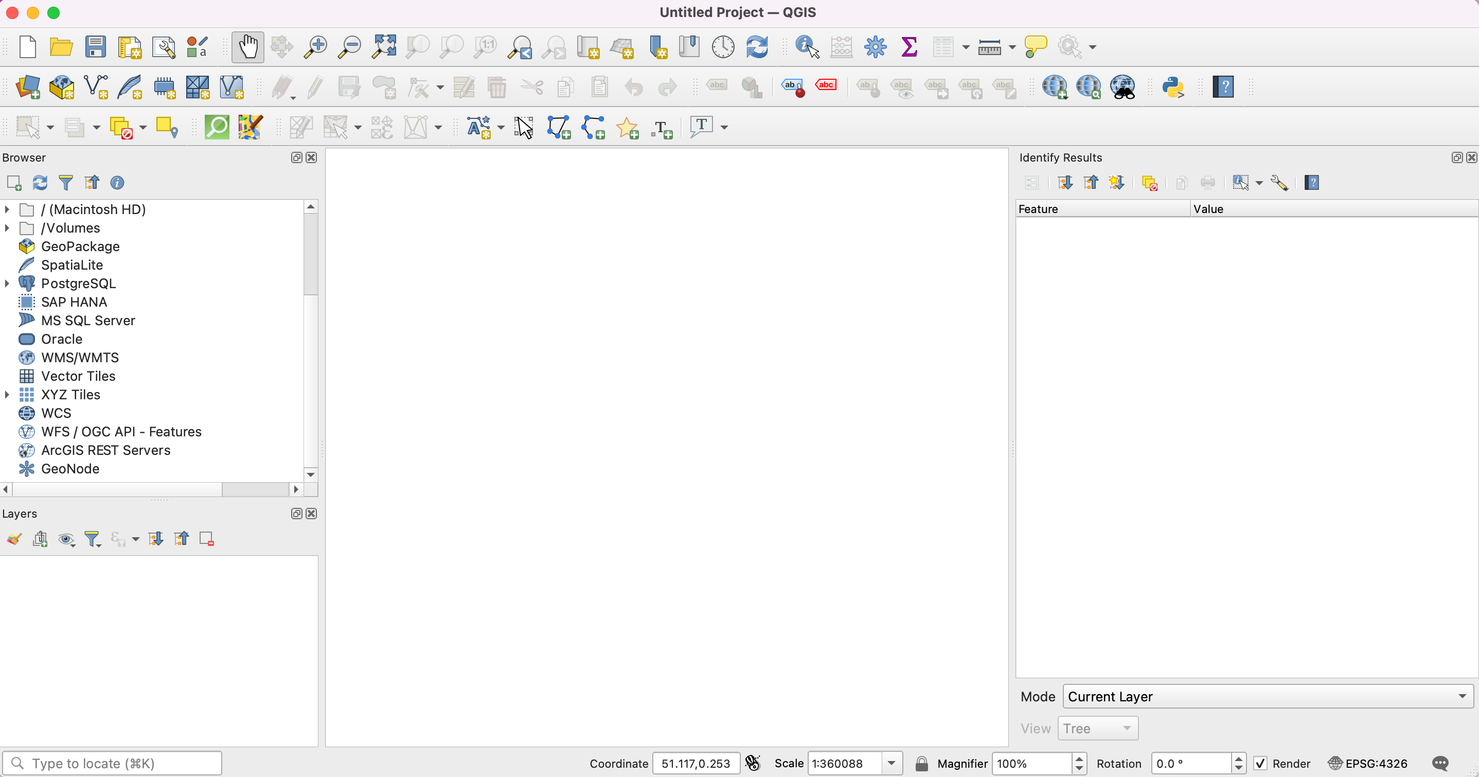
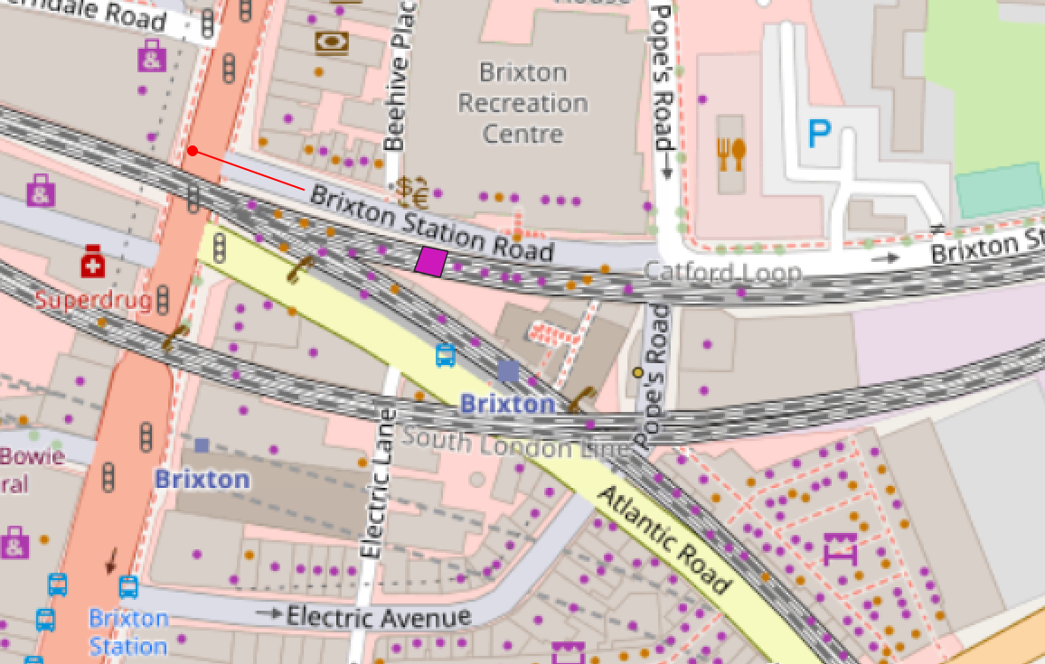
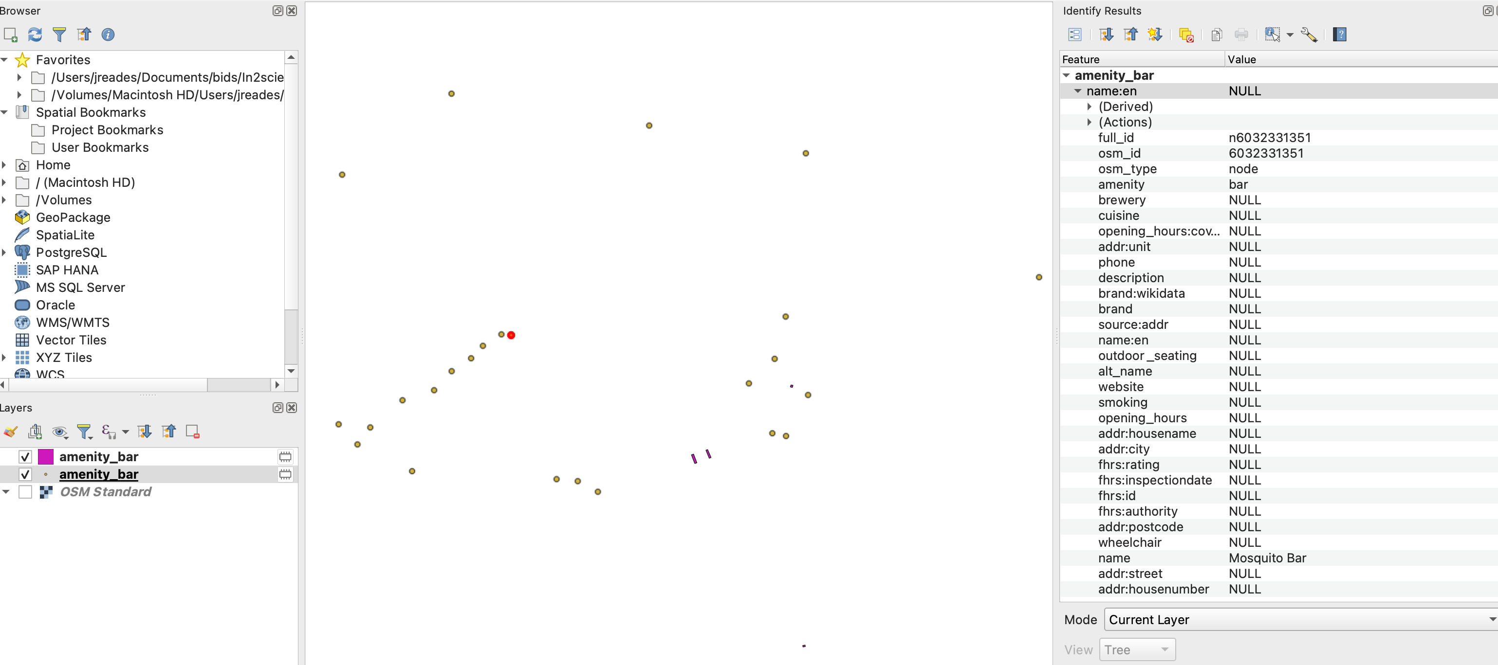
Select one of the two new amenity_bar layers by clicking on it in the Layers area, and then pick the ‘info’ button (it’s an arrow with an i in a blue circle). See what information you can find out about some of the bars!
Notice that you can only get information for a layer that you’ve selected in the Layers panel. In the screenshot below amenity_bar with a circle icon is selected so I can only use the ‘info’ button to get more information about data in that layer.
2.6 Questions
- Why do you think that two layers named
amenity_barwere added to QGIS? Hint: try right-clicking on each one in turn and pickingZoom to Layersthen turn each amenity layer on and off in turn while seeing if you can spot the difference! - Using the information button, can you think about other ways that you might be able to find Brixton bars? Hint: while using
amenity=baris likely the best way, it’s definitely not the only way! Are there other attributes that might help? - Using the tip below, see if you can use multiple criteria in your QuickOSM search to find Yoga Studios in the area. Hint: this will be a Boolean logic problem that you would encounter in any programming class.
- Using what you’ve been discussing in previous classes together with some ideas contained in this Twitter thread see if you can come up with some other QuickOSM queries to pull data on possible markers of gentrification in the Brixton area.
If you’re not sure how to find something then check the OSM Wiki. For instance, if you Google OSM Wiki yoga you will get tips on searching for yoga studios using synonyms.
3 Get the Remaining Data
OK, now let’s get the rest of data that we need for this practical. I’ve (partially) prepared some data for you so that you don’t have to track everything down yourselves.
There are three files you need:
Once these have been downloaded, I would suggest moving all of these to your ‘Documents’ folder before double-clicking them to unzip the Zip archives. The GeoPackage (.gpkg) does not need to be unzipped.
4 Add the Boroughs
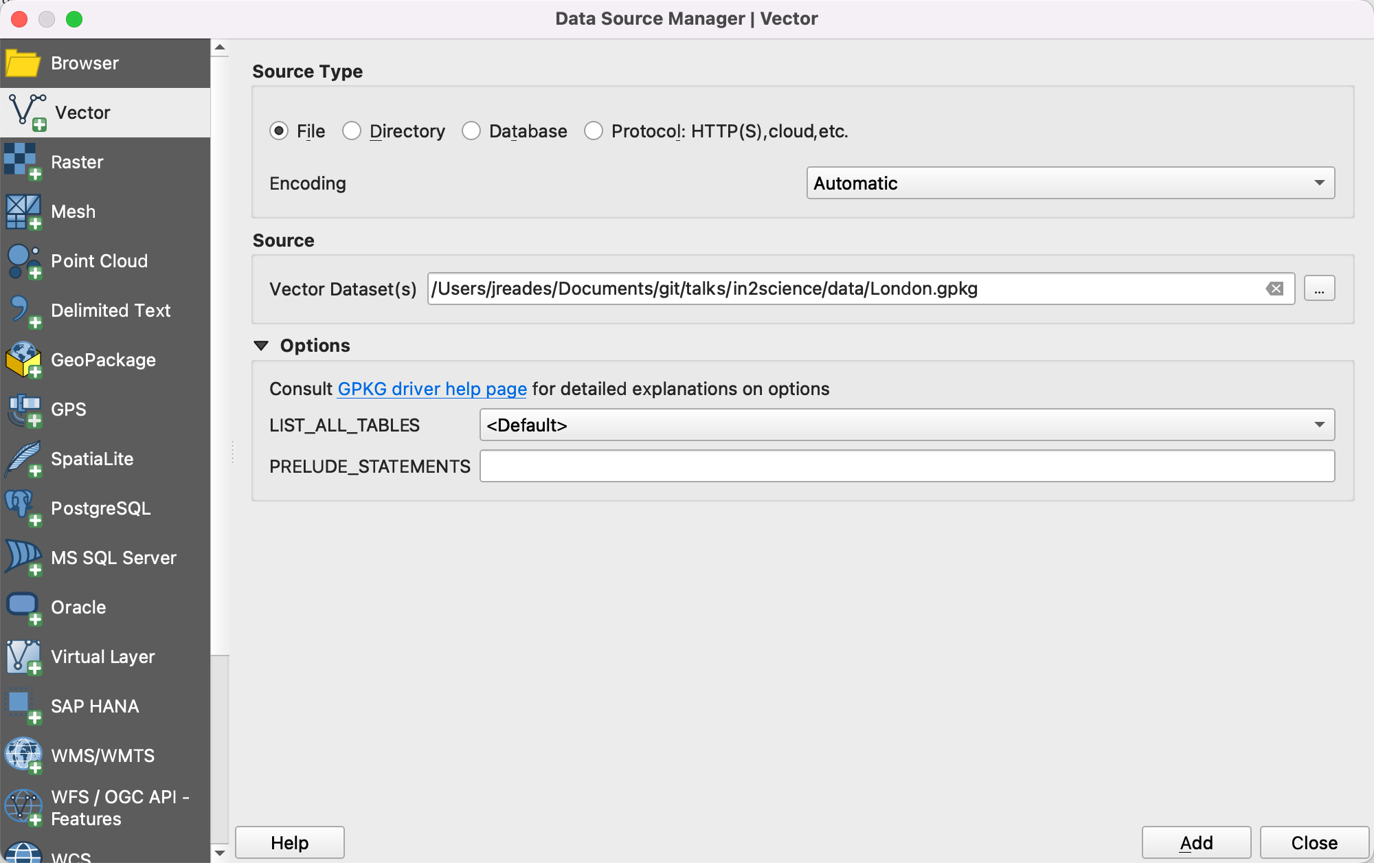
‘Vector’ data that is already ready to display on a map is easy to add to QGIS. Under the Layer menu option select Add Layer then Add Vector Layer as shown below.
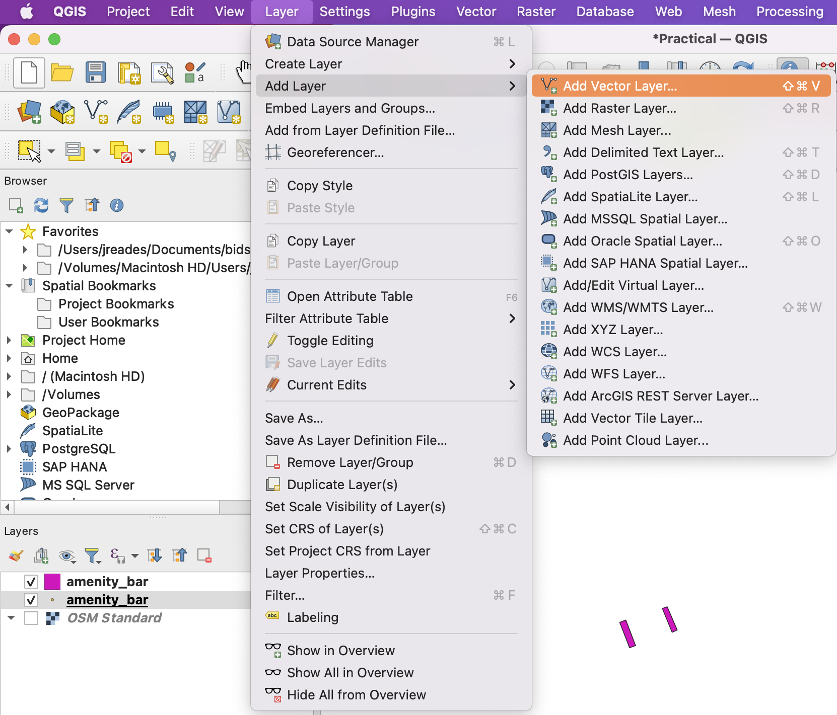
This will bring up the Add Vector Layer popup and you then click on the ... to navigate to where you saved London.gpkg. Select this, click Add, and see what happens!
Hmmmmm, what is this?
![]()
For now, just take the selected the option, click OK to make the Transform popup go away, and then click Close to make the Add Vector Layer popup disappear.
You will now need to zoom out quite a bit to see what you’ve done!
4.1 Rearranging Layers
Take a close look at the Layers area in QGIS. If London has ended up in between your amenity... layers you may want to rearrange things so that it’s at the bottom, just above the OSM Standard layer. You do that by clicking-and-dragging as shown here:
4.2 Styling Boroughs
Now that you can clearly see both London and any OSM layers:
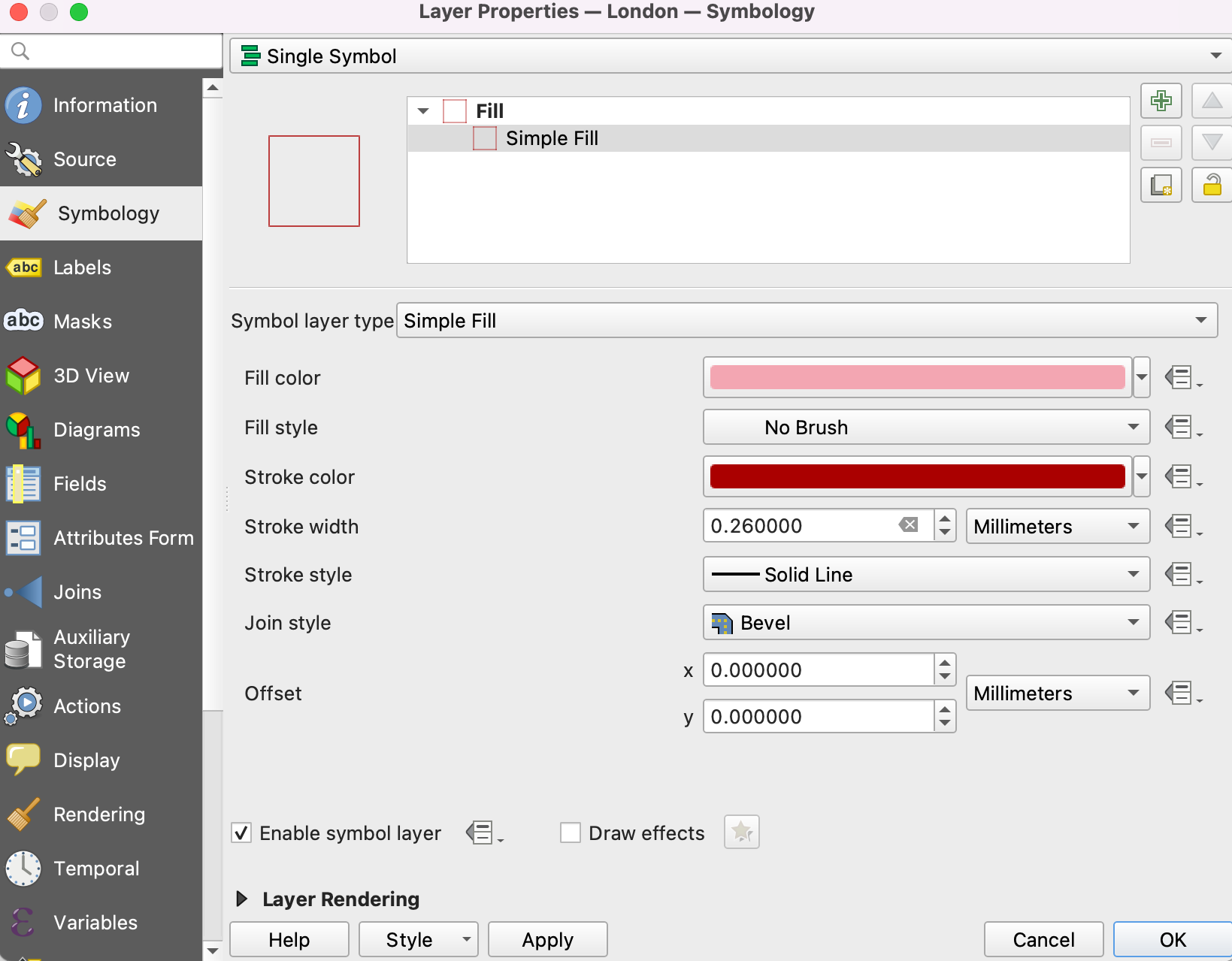
- Right-click (Ctrl+Click on a Mac) on the layer and pick
Propertiesto open theLayer Propertiespopup - Pick
Symbologyfrom the area on the left. - Click on the area labelled
Simple Fill(see below). - Change the
Fill colortoNo brush - Change the
Stroke colorto a dark red.
Your Layer Properties should look something like this:
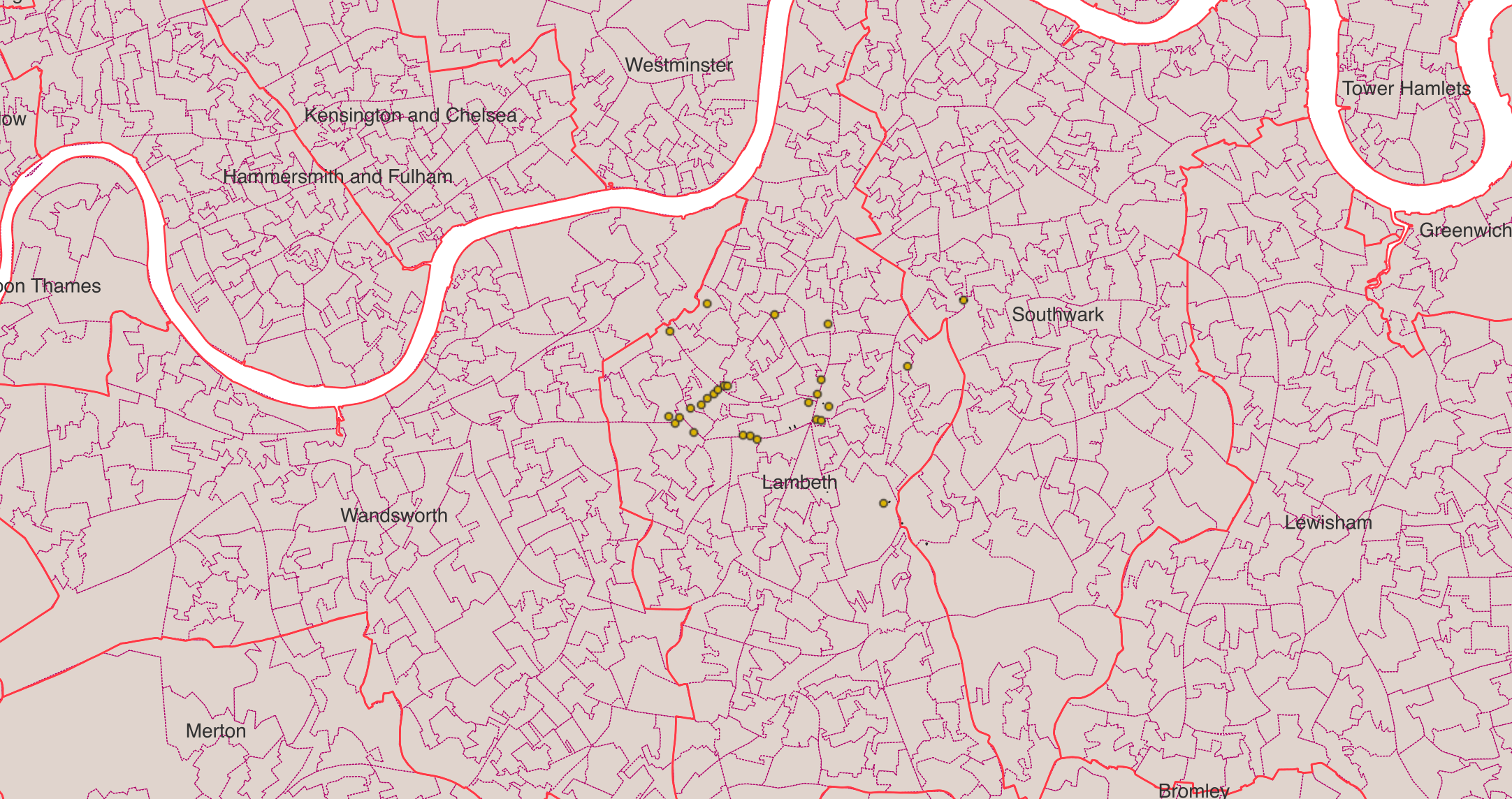
Click OK and have a close look at your map of London. You should now see the boroughs outlined in red with the OSM Standard layer visible ‘behind’ and any QuickOSM layers visible ‘on top’.
4.3 Labelling Boroughs
Right-click on the London layer again to bring up Properties, but this time pick Labels from the left-hand side:
- Change
No labelstoSingle labels. - The
Valueshould already be set toNAME(which is what we want) - Change the font size to 14 (from 10.0000).
- Click
OKand you should now see labels for each borough.
5 Adding LSOAs
Find and double-click on LSOA_2011_London_gen_MHW.shp. Your computer might add the layer to your current QGIS document, or the computer might just say that it has no idea what to do. The better way to add data is using the Add Vector Layer menu option or short-cut (again).
- From
LayerselectAdd Vector Layer - You’ll see that you’re in the Data Source Manager popup with the
Vectoroption selected. - Again, click on the
...(to the right ofVector Dataset(s)). - And navigate to where you unzipped the unzipped LSOA files.
- Select
LSOA_2011_London_gen_MHW.shp - Click
Add
If the LSOA layer has appeared on top of the London boroughs layer then just drag-and-drop to rearrange the order so that the LSOAs are ‘behind’ the boroughs!
See if you can change the style of the LSOA layer to something like the image below. Remember that you do this through Layer Properties!
6 Let’s Talk Data
OK, finally we need to add the ‘real’ data to the map! The CSV file that you downloaded and unzipped into Census_2001_2011.csv contains the following attributes:
- Median House Prices in 2001 & 2011
- Median Household Income in 2001 & 2011
- Percentage with Level 4+ NVQ Qualifications in 2001 & 2011
- Percentage of Higher and Lower Managerial Workers in 2001 & 2011
The first few rows look like this:
| lsoacd | House Prices 2001 | Percentage with Level 4+ Qualifications 2001 | Percentage of Knowledge Workers 2001 | Household Income 2001 | House Prices 2011 | Percentage with Level 4+ Qualifications 2011 | Percentage of Knowledge Workers 2011 | Household Income 2011 |
|---|---|---|---|---|---|---|---|---|
| E01000001 | 255450 | 72.3120169 | 86.3765374 | 45630 | 504999.5 | 77.5555556 | 88.6609071 | 65520 |
| E01000002 | 244000 | 68.3584457 | 86.0125261 | 44970 | 525000 | 79.195669 | 87.3626374 | 66300 |
| E01000003 | 175000 | 50.3252033 | 65.6019656 | 36330 | 350000 | 56.8438003 | 72.9057592 | 54140 |
| E01000005 | 132000 | 31.3237221 | 47.1794872 | 31530 | 300000 | 34.4701583 | 46.2184874 | 46740 |
| E01032739 | 230000 | 64.6043162 | 80.6902998 | 44710 | 447500 | 73.6465781 | 84.1269841 | 62460 |
The lsoacd is the key field here since it tells us what LSOA (a.k.a. small neighbourhood-type area) is being ‘talked about’ here.
Questions:
Thinking as a scientist about what we’ve discussed in earlier sessions, answer the following questions about the data and how they might connect to questions about gentrification:
- What does each row represent?
- What does each column represent?
- What is the significance of 2001 and 2011 as dates for providing us with data? The answer is in the name of the file…
- Why did I provide you with median instead of mean house prices and household incomes? This is a maths question and your hint is: \(\sigma^{2} = \frac{\sum(x-\bar{x})^{2}}{N}\).
- Why did I provide you with median household income instead of median individual income? This is a measurment bias question…
- What is a Level 4 (or more) NVQ and why would I include this in the file? Use Google to find this out…
- Why would the share of Higher and Lower Managerial workers be included? You might need to look at the National Statistics Socio-Economic Classification.
7 Add the Census Data
Click on the Layer menu and then pick Data Source Manager (DSM) in the menu at the top of your screen. This will bring up the dialogue box below, and then pick Delimited Text (as in the image below).
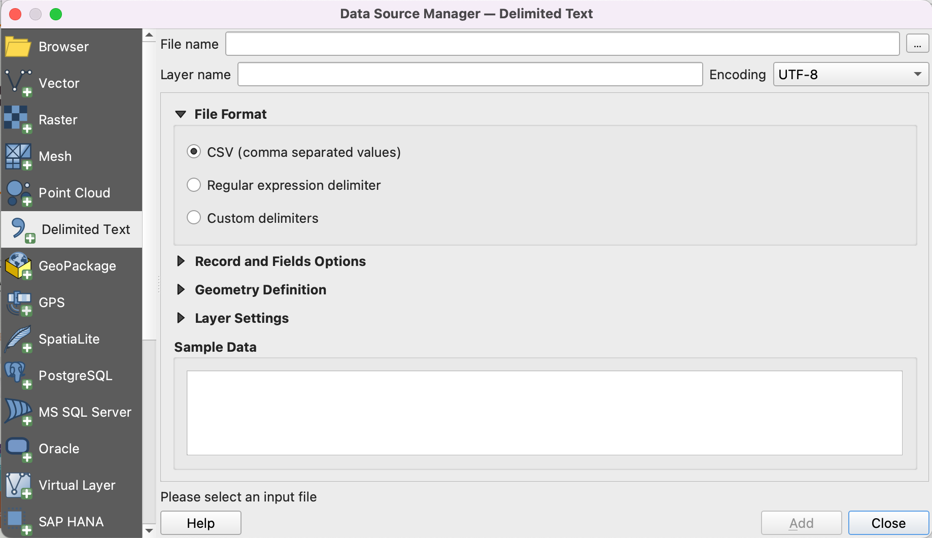
You now need to follow these steps carefully:
- Make sure that
Delimitted Textis selected in the left-hand area. - Click on the
...to the right of ‘File name’ in the DSM manager. - Find where you saved the
Census_2001_2011.csvfile, select it, and pickOpen.
You can see that there are data types in the Sample Data area (double, string, etc.). We’ll accept the defaults that QGIS has chosen for us, but we could, for instace, tell QGIS to use integers instead of double-precision floats for House Prices since people don’t pay £157,340.26 for a house! Before you click ‘Add’, we need to tell QGIS that there’s no geometry (i.e. nothing to actually map):
- Click on the black triangle next to
Geometry Definitionand make sure thatNo geometry (attribute only table)is selected. - Now click
Add, thenCloseonce the DSM turns blank and…
Nothing has changed! WTF???
The reason we can’t see any changes on the map is that we’ve just added data, not mapped data.
8 Joining Data
This is the last thing we want to do before breaking, and it’s the hardest. We need to help QGIS to show, say, house prices in 2001 by linking (joining) the CSV data that we just added to the LSOA layer that we added earlier.
There’s a set of videos to show you how it’s done.
8.1 Part 1: Creating the Join
Step-by-step this is:
- Right-click on the LSOA layer and select
Properties. - Select
Joinsfrom the left-hand side of the Layers popup. - Click the
+button. - In the
Add Vector Joinpopup:- Change the
Join layerto the CSV file. - The
Join Fieldshould change tolsoacdautomatically, but in case it doesn’t… - The
Target Fieldshould already beLSOA11CD, but in case it isn’t…
- Change the
- Click
OK
Again, nothing seems to have changed!
8.2 Part 2: Checking the Join
If nothing has changed, how do we know if it ‘worked’, or even what the heck happened:
- Right-click on the LSOA layer again and select
Open Attribute Table. - In the resulting popup, scroll all the way to the right.
- You should see that the columns from the Census data CSV file have been added to the LSOA data file, row-by-row!
Close the table now that we’ve checked the data was added.
8.3 Part 3: Changing the Symbology
Now let’s see what we can do with our joined data:
- Select the
Layer Propertiesand pickSymbologyfrom the left-hand side of the popup. - At the top of the popup change
Single SymboltoGraduated, which means that the colour will now depend on a data value! - Set the
Valueto the 2001 house price data. - Change the
Color ramp(if you like) - Change the number of
Classes(if you like) - Change the
Mode(if you like) - Click
Classifyto see your changes. - Click
Applyand thenOK
Now your map looks different!
8.4 Part 4: Checking the Results
In this last part we just want to check the results make some kind of sense. In my video, using Rocket colour ramp, the lightest colours are the highest values. Here is use the ‘info’ button again to find the highest value in the data set and check based on the colour and check what the price was in 2001.
9 Save & Get Coffee
One last thing: let’s save our work.
- The join is temporary (you will lose it if you shut down QGIS) so let’s save a new layer.
- Right-click on the LSOA layer.
- Select
ExportandSave Features As... - Click on the
...next toFile nameand choose a place to save your new file. We will use theGeoPackageformat because it’s easy to save/load. - Make sure that
Add saved file to mapis ticked at the bottom of the popup. - Click
OKand you should see a green feedback message appear after a few seconds sayingLayer Exported: Success...and a new layer without any colouring appear in the Layers area of QGIS.
- Copy the layer style:
- We don’t want to have to recreate the colour-scheme that we created above again, so let’s copy+paste!
- Right-click on the original LSOA layer and pick
StylesthenCopy styleandAll style categories. - Now select the new LSOA layer and pick
StylesthenPaste styleandAll style categories. - Both layers should now have the same styles: how could you check this using the Layers options in QGIS?
- Save the QGIS project by clicking on the
Saveicon and giving your project a name.
10 Congratulations!
Congrats, you’ve created your first choropleth map in addition to running a query on a spatial database, and doing a non-spatial database join.