<class 'pandas.core.frame.DataFrame'>
['State', 'District', 'Subdistt', 'Town/Village', 'Ward', 'EB', 'Level', 'Name', 'TRU', 'No_HH', 'TOT_P', 'TOT_M', 'TOT_F', 'P_06', 'M_06', 'F_06', 'P_SC', 'M_SC', 'F_SC', 'P_ST', 'M_ST', 'F_ST', 'P_LIT', 'M_LIT', 'F_LIT', 'P_ILL', 'M_ILL', 'F_ILL', 'TOT_WORK_P', 'TOT_WORK_M', 'TOT_WORK_F', 'MAINWORK_P', 'MAINWORK_M', 'MAINWORK_F', 'MAIN_CL_P', 'MAIN_CL_M', 'MAIN_CL_F', 'MAIN_AL_P', 'MAIN_AL_M', 'MAIN_AL_F', 'MAIN_HH_P', 'MAIN_HH_M', 'MAIN_HH_F', 'MAIN_OT_P', 'MAIN_OT_M', 'MAIN_OT_F', 'MARGWORK_P', 'MARGWORK_M', 'MARGWORK_F', 'MARG_CL_P', 'MARG_CL_M', 'MARG_CL_F', 'MARG_AL_P', 'MARG_AL_M', 'MARG_AL_F', 'MARG_HH_P', 'MARG_HH_M', 'MARG_HH_F', 'MARG_OT_P', 'MARG_OT_M', 'MARG_OT_F', 'MARGWORK_3_6_P', 'MARGWORK_3_6_M', 'MARGWORK_3_6_F', 'MARG_CL_3_6_P', 'MARG_CL_3_6_M', 'MARG_CL_3_6_F', 'MARG_AL_3_6_P', 'MARG_AL_3_6_M', 'MARG_AL_3_6_F', 'MARG_HH_3_6_P', 'MARG_HH_3_6_M', 'MARG_HH_3_6_F', 'MARG_OT_3_6_P', 'MARG_OT_3_6_M', 'MARG_OT_3_6_F', 'MARGWORK_0_3_P', 'MARGWORK_0_3_M', 'MARGWORK_0_3_F', 'MARG_CL_0_3_P', 'MARG_CL_0_3_M', 'MARG_CL_0_3_F', 'MARG_AL_0_3_P', 'MARG_AL_0_3_M', 'MARG_AL_0_3_F', 'MARG_HH_0_3_P', 'MARG_HH_0_3_M', 'MARG_HH_0_3_F', 'MARG_OT_0_3_P', 'MARG_OT_0_3_M', 'MARG_OT_0_3_F', 'NON_WORK_P', 'NON_WORK_M', 'NON_WORK_F']Pandas
Jon Reades

Why Pandas?
Pandas is probably (together with scipy, numpy, and sklearn) the main reason that Python has become popular for data science. According to ‘Learn Data Sci’ it accounts for 1% of all Stack Overflow question views!
You will want to bookmark these:
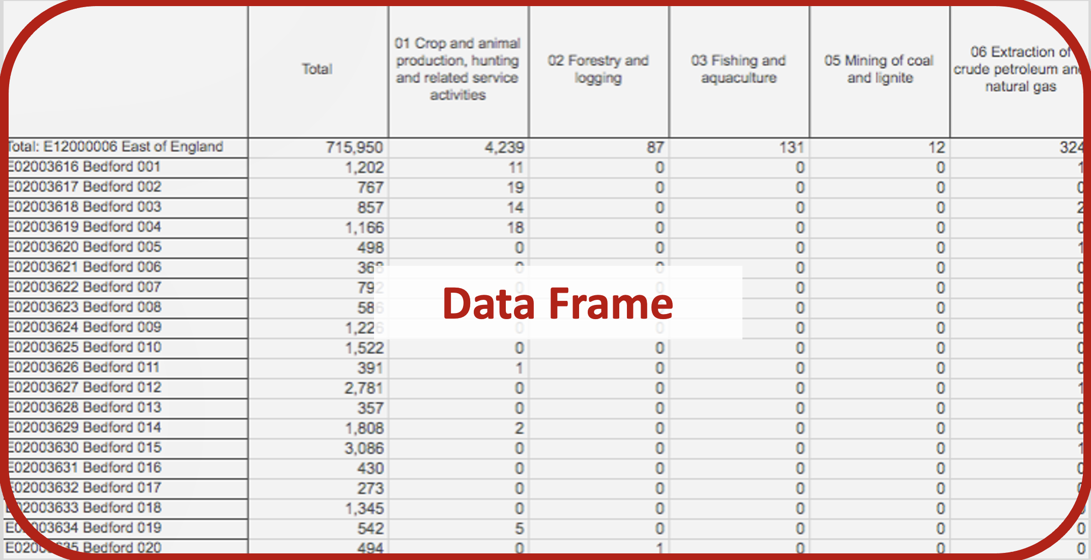
Pandas Terminology (Data Frame)
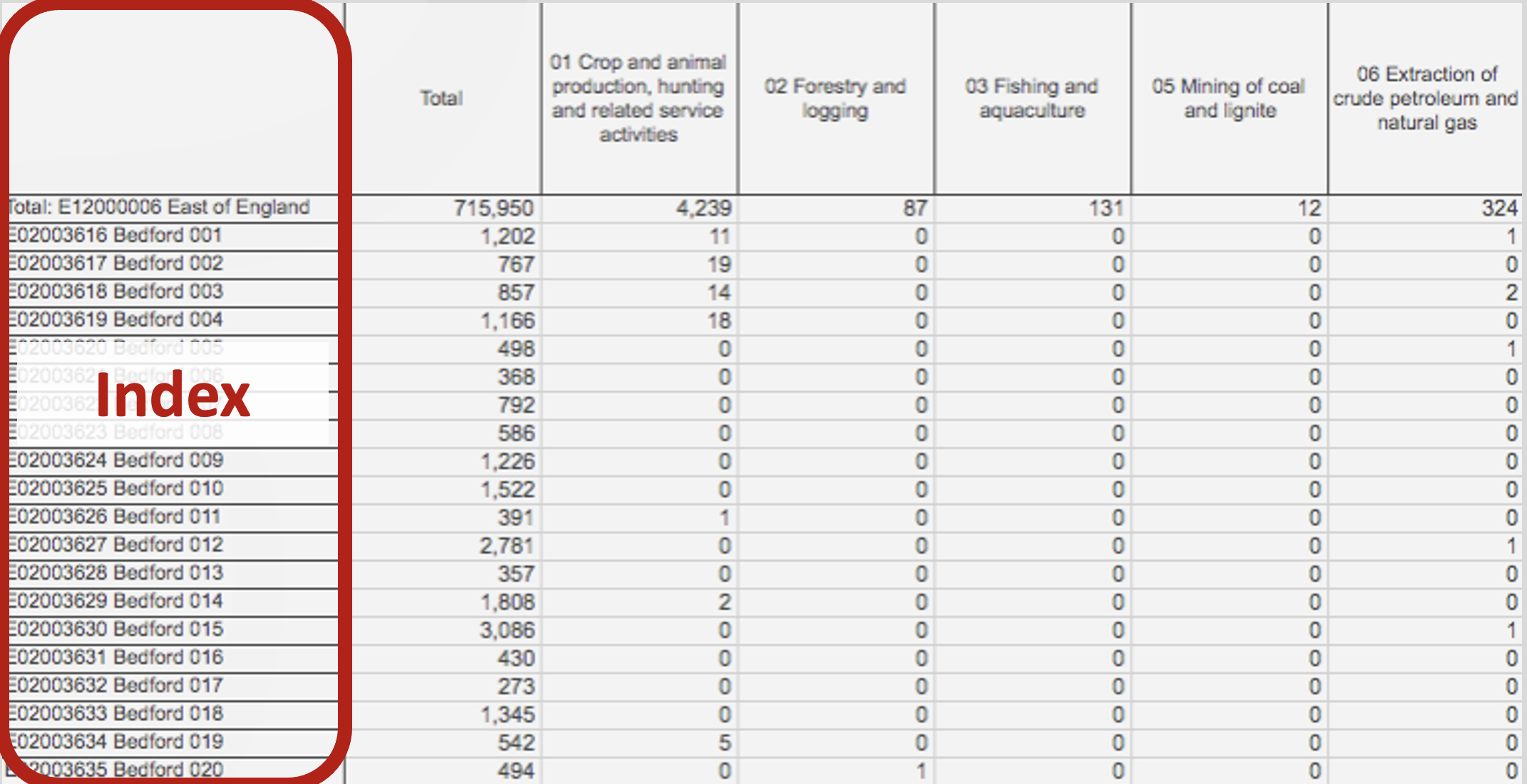
Pandas Terminology (Index)
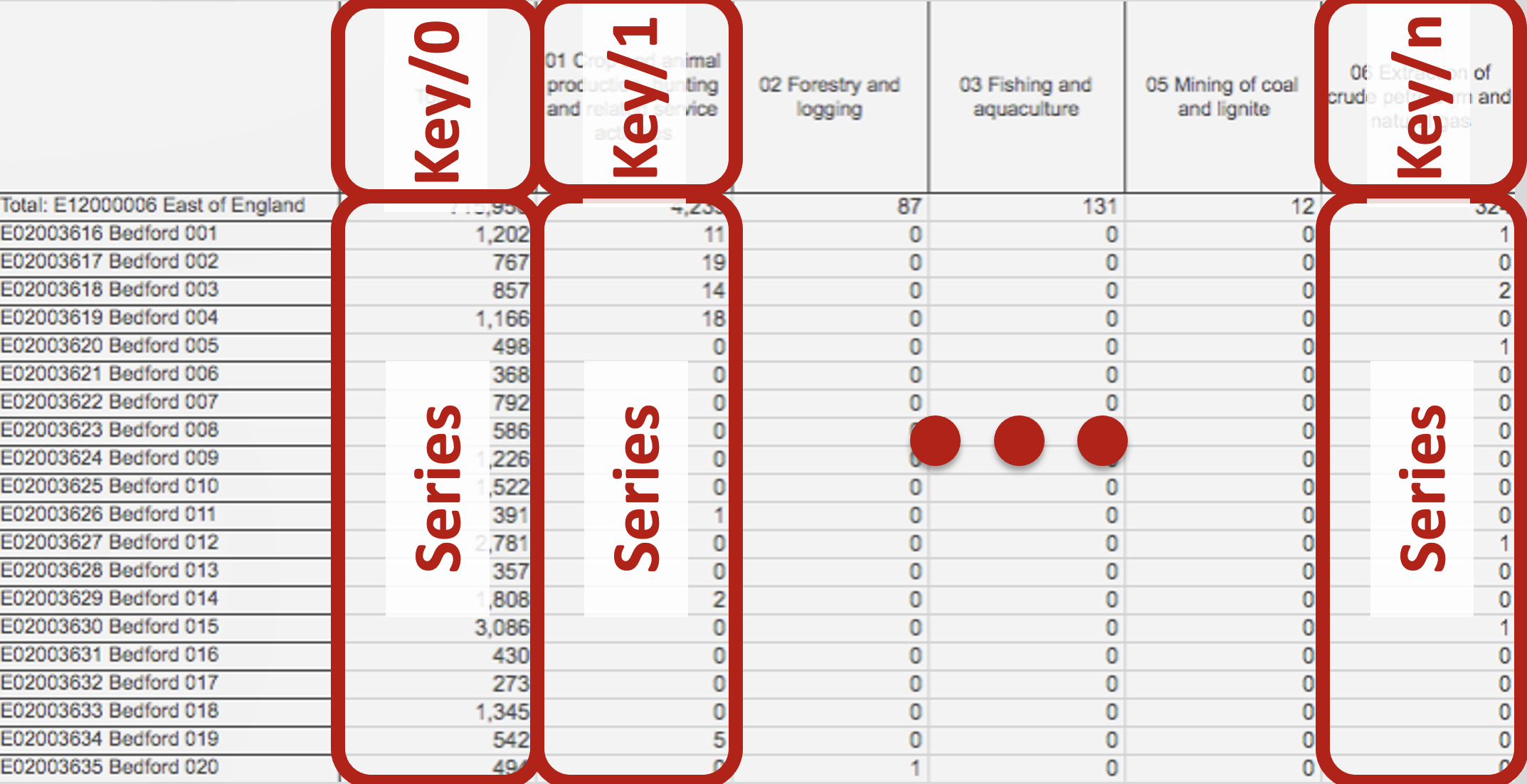
Pandas Terminology (Series)
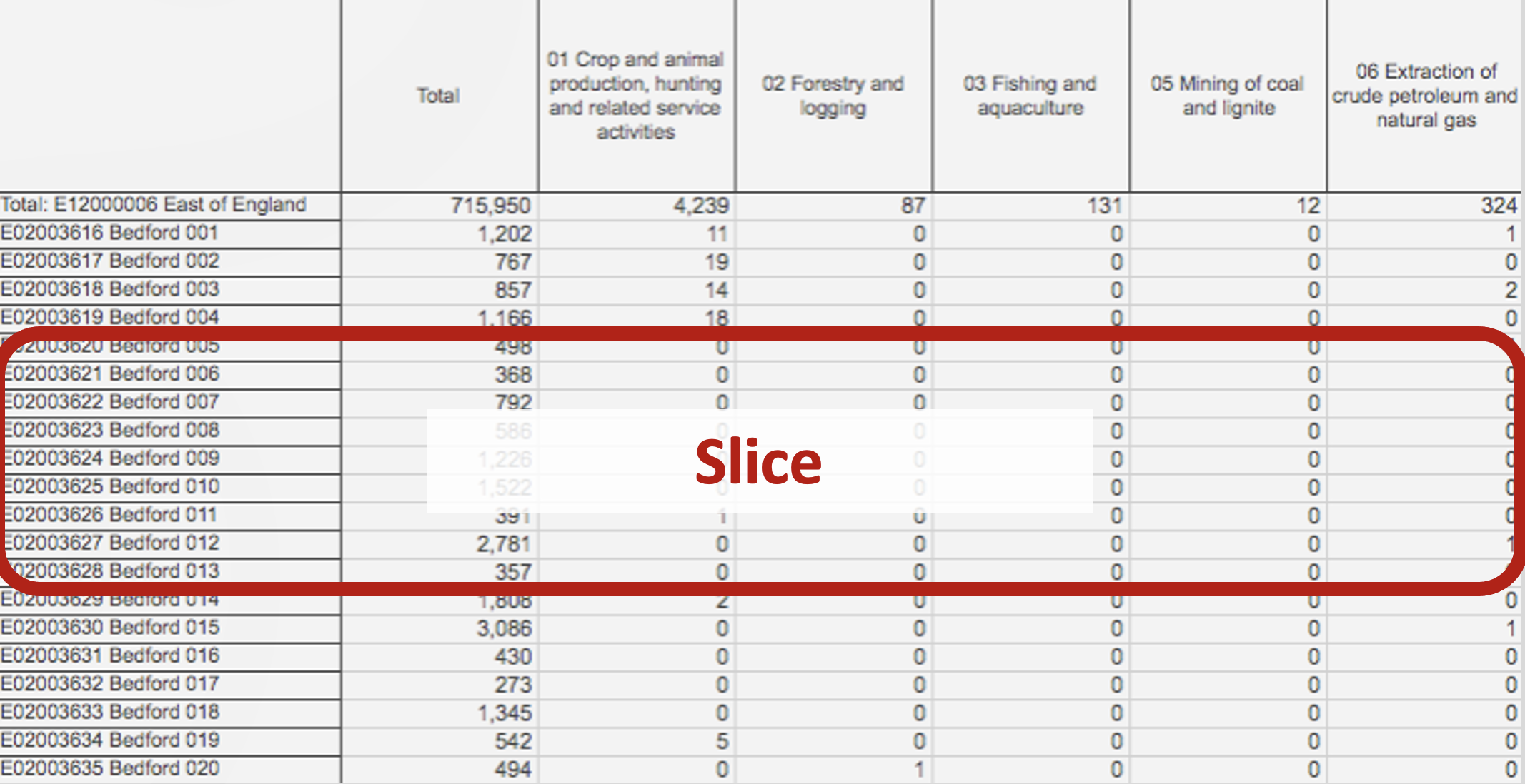
Pandas Terminology (Slice)
Using Pandas
Here’s code to read a (remote) CSV file:
import pandas as pd         # import package
url='https://orca.casa.ucl.ac.uk/~jreades/jaipur/population.csv.gz'
df = pd.read_csv(url)       # load a (remote) CSV
print(type(df))             # not a 'simple' data type
print(df.columns.to_list()) # column namesSummarise a Data Frame
Statistical summarisation.
| State | District | Subdistt | Town/Village | Ward | EB | No_HH | TOT_P | TOT_M | TOT_F | ... | MARG_AL_0_3_F | MARG_HH_0_3_P | MARG_HH_0_3_M | MARG_HH_0_3_F | MARG_OT_0_3_P | MARG_OT_0_3_M | MARG_OT_0_3_F | NON_WORK_P | NON_WORK_M | NON_WORK_F | |
|---|---|---|---|---|---|---|---|---|---|---|---|---|---|---|---|---|---|---|---|---|---|
| count | 2561.0 | 2561.0 | 2561.000000 | 2561.000000 | 2561.000000 | 2561.0 | 2.561000e+03 | 2.561000e+03 | 2.561000e+03 | 2.561000e+03 | ... | 2561.000000 | 2561.000000 | 2561.000000 | 2561.000000 | 2561.000000 | 2561.000000 | 2561.000000 | 2.561000e+03 | 2.561000e+03 | 2.561000e+03 |
| mean | 8.0 | 110.0 | 543.976962 | 169642.691527 | 2.311207 | 0.0 | 2.561084e+03 | 1.430145e+04 | 7.489366e+03 | 6.812087e+03 | ... | 13.509567 | 8.444748 | 3.001171 | 5.443577 | 66.545881 | 27.736431 | 38.809449 | 9.049970e+03 | 3.776792e+03 | 5.273178e+03 |
| std | 0.0 | 0.0 | 19.015389 | 239933.613990 | 8.628916 | 0.0 | 3.293322e+04 | 1.815688e+05 | 9.511259e+04 | 8.645723e+04 | ... | 189.164285 | 106.745661 | 38.197017 | 69.027967 | 851.119683 | 350.089056 | 516.492442 | 1.158499e+05 | 4.771246e+04 | 6.835303e+04 |
| min | 8.0 | 110.0 | 0.000000 | 0.000000 | 0.000000 | 0.0 | 0.000000e+00 | 0.000000e+00 | 0.000000e+00 | 0.000000e+00 | ... | 0.000000 | 0.000000 | 0.000000 | 0.000000 | 0.000000 | 0.000000 | 0.000000 | 0.000000e+00 | 0.000000e+00 | 0.000000e+00 |
| 25% | 8.0 | 110.0 | 542.000000 | 79596.000000 | 0.000000 | 0.0 | 9.500000e+01 | 6.010000e+02 | 3.100000e+02 | 2.870000e+02 | ... | 0.000000 | 0.000000 | 0.000000 | 0.000000 | 0.000000 | 0.000000 | 0.000000 | 3.120000e+02 | 1.570000e+02 | 1.520000e+02 |
| 50% | 8.0 | 110.0 | 545.000000 | 80236.000000 | 0.000000 | 0.0 | 1.700000e+02 | 1.064000e+03 | 5.530000e+02 | 5.120000e+02 | ... | 0.000000 | 0.000000 | 0.000000 | 0.000000 | 2.000000 | 1.000000 | 1.000000 | 6.050000e+02 | 2.870000e+02 | 3.110000e+02 |
| 75% | 8.0 | 110.0 | 548.000000 | 80873.000000 | 0.000000 | 0.0 | 3.170000e+02 | 1.934000e+03 | 1.010000e+03 | 9.200000e+02 | ... | 2.000000 | 1.000000 | 0.000000 | 0.000000 | 11.000000 | 4.000000 | 6.000000 | 1.148000e+03 | 5.280000e+02 | 6.230000e+02 |
| max | 8.0 | 110.0 | 550.000000 | 800523.000000 | 77.000000 | 0.0 | 1.177096e+06 | 6.626178e+06 | 3.468507e+06 | 3.157671e+06 | ... | 6775.000000 | 4002.000000 | 1405.000000 | 2597.000000 | 32114.000000 | 13016.000000 | 19098.000000 | 4.161285e+06 | 1.753560e+06 | 2.407725e+06 |
8 rows × 91 columns
Data types and memory usage.
<class 'pandas.core.frame.DataFrame'>
RangeIndex: 2561 entries, 0 to 2560
Data columns (total 94 columns):
 #   Column          Non-Null Count  Dtype
---  ------          --------------  -----
 0   State           2561 non-null   int64
 1   District        2561 non-null   int64
 2   Subdistt        2561 non-null   int64
 3   Town/Village    2561 non-null   int64
 4   Ward            2561 non-null   int64
 5   EB              2561 non-null   int64
 6   Level           2561 non-null   object
 7   Name            2561 non-null   object
 8   TRU             2561 non-null   object
 9   No_HH           2561 non-null   int64
 10  TOT_P           2561 non-null   int64
 11  TOT_M           2561 non-null   int64
 12  TOT_F           2561 non-null   int64
 13  P_06            2561 non-null   int64
 14  M_06            2561 non-null   int64
 15  F_06            2561 non-null   int64
 16  P_SC            2561 non-null   int64
 17  M_SC            2561 non-null   int64
 18  F_SC            2561 non-null   int64
 19  P_ST            2561 non-null   int64
 20  M_ST            2561 non-null   int64
 21  F_ST            2561 non-null   int64
 22  P_LIT           2561 non-null   int64
 23  M_LIT           2561 non-null   int64
 24  F_LIT           2561 non-null   int64
 25  P_ILL           2561 non-null   int64
 26  M_ILL           2561 non-null   int64
 27  F_ILL           2561 non-null   int64
 28  TOT_WORK_P      2561 non-null   int64
 29  TOT_WORK_M      2561 non-null   int64
 30  TOT_WORK_F      2561 non-null   int64
 31  MAINWORK_P      2561 non-null   int64
 32  MAINWORK_M      2561 non-null   int64
 33  MAINWORK_F      2561 non-null   int64
 34  MAIN_CL_P       2561 non-null   int64
 35  MAIN_CL_M       2561 non-null   int64
 36  MAIN_CL_F       2561 non-null   int64
 37  MAIN_AL_P       2561 non-null   int64
 38  MAIN_AL_M       2561 non-null   int64
 39  MAIN_AL_F       2561 non-null   int64
 40  MAIN_HH_P       2561 non-null   int64
 41  MAIN_HH_M       2561 non-null   int64
 42  MAIN_HH_F       2561 non-null   int64
 43  MAIN_OT_P       2561 non-null   int64
 44  MAIN_OT_M       2561 non-null   int64
 45  MAIN_OT_F       2561 non-null   int64
 46  MARGWORK_P      2561 non-null   int64
 47  MARGWORK_M      2561 non-null   int64
 48  MARGWORK_F      2561 non-null   int64
 49  MARG_CL_P       2561 non-null   int64
 50  MARG_CL_M       2561 non-null   int64
 51  MARG_CL_F       2561 non-null   int64
 52  MARG_AL_P       2561 non-null   int64
 53  MARG_AL_M       2561 non-null   int64
 54  MARG_AL_F       2561 non-null   int64
 55  MARG_HH_P       2561 non-null   int64
 56  MARG_HH_M       2561 non-null   int64
 57  MARG_HH_F       2561 non-null   int64
 58  MARG_OT_P       2561 non-null   int64
 59  MARG_OT_M       2561 non-null   int64
 60  MARG_OT_F       2561 non-null   int64
 61  MARGWORK_3_6_P  2561 non-null   int64
 62  MARGWORK_3_6_M  2561 non-null   int64
 63  MARGWORK_3_6_F  2561 non-null   int64
 64  MARG_CL_3_6_P   2561 non-null   int64
 65  MARG_CL_3_6_M   2561 non-null   int64
 66  MARG_CL_3_6_F   2561 non-null   int64
 67  MARG_AL_3_6_P   2561 non-null   int64
 68  MARG_AL_3_6_M   2561 non-null   int64
 69  MARG_AL_3_6_F   2561 non-null   int64
 70  MARG_HH_3_6_P   2561 non-null   int64
 71  MARG_HH_3_6_M   2561 non-null   int64
 72  MARG_HH_3_6_F   2561 non-null   int64
 73  MARG_OT_3_6_P   2561 non-null   int64
 74  MARG_OT_3_6_M   2561 non-null   int64
 75  MARG_OT_3_6_F   2561 non-null   int64
 76  MARGWORK_0_3_P  2561 non-null   int64
 77  MARGWORK_0_3_M  2561 non-null   int64
 78  MARGWORK_0_3_F  2561 non-null   int64
 79  MARG_CL_0_3_P   2561 non-null   int64
 80  MARG_CL_0_3_M   2561 non-null   int64
 81  MARG_CL_0_3_F   2561 non-null   int64
 82  MARG_AL_0_3_P   2561 non-null   int64
 83  MARG_AL_0_3_M   2561 non-null   int64
 84  MARG_AL_0_3_F   2561 non-null   int64
 85  MARG_HH_0_3_P   2561 non-null   int64
 86  MARG_HH_0_3_M   2561 non-null   int64
 87  MARG_HH_0_3_F   2561 non-null   int64
 88  MARG_OT_0_3_P   2561 non-null   int64
 89  MARG_OT_0_3_M   2561 non-null   int64
 90  MARG_OT_0_3_F   2561 non-null   int64
 91  NON_WORK_P      2561 non-null   int64
 92  NON_WORK_M      2561 non-null   int64
 93  NON_WORK_F      2561 non-null   int64
dtypes: int64(91), object(3)
memory usage: 1.8+ MB
Accessing a Series
Jupyter Formatting
Pandas is also ‘Jupyter-aware’, meaning that output can displayed directly in Jupyter and Quarto in ‘fancy’ ways:
Nosing Around
df.head(3)                       # First 3 rows of df
df[['TOT_F','F_SC']].tail(3)     # Last 3 rows of selected columns
df.sample(frac=0.3)              # A random 30% sample
df.sample(3, random_state=42)    # A random sample of 3 with a seed
df.sample(3, random_state=42)    # Same sample!
Head and tail are used on the Command Line. Random sampling with seeds is covered in my talk on Randomness. We’ve even got Lists of Lists, which is a really basic data structure!
Data Frames vs Series
Pandas operates on two principles:
- Any operation on a Data Frame returns a Data Frame.
- Any operation on a Series returns a Series.
Putting These Ideas Together
# Returns a series
print(type(df.TOT_F - 1))
# Saves returned series as a new column
df['smaller'] = df.TOT_F - 1
print(df[['TOT_F','smaller']].head(3))
# Returns a new data frame w/o the dropped column
print(type(df.drop(columns=['smaller'])))
<class 'pandas.core.series.Series'>
TOT_F smaller
0 3157671 3157670
1 1511407 1511406
2 1646264 1646263
<class 'pandas.core.frame.DataFrame'>What Can We Do?
Chaining
Operations on a Data Frame return a DataFrame and operations on a Series return a Series, allowing us to ‘chain’ steps together:
df.sort_values(by=['TOT_P','TOT_M'], ascending=False).head(20).sample(frac=0.5).median(numeric_only=True)State 8.0
District 110.0
Subdistt 545.5
Town/Village 0.0
Ward 0.0
...
MARG_OT_0_3_F 1140.5
NON_WORK_P 268462.0
NON_WORK_M 121100.0
NON_WORK_F 147362.0
smaller 205513.0
Length: 92, dtype: float64Selection
# Returns a selection (Boolean series)
df['TOT_P']>5000
# Data frame of records matching selection
df[ df['TOT_P']>5000 ]

# Calculations on a slice (returns mean centroid!)
df[df['TOT_P']>5000][['TOT_M','TOT_F']].mean()
You can link several conditions using & (and) and | (or).
Now we can automate… data anlysis!
Dealing with Types
A Data Series can only be of one type:
| Pandas Dtype | Python Type | Usage |
|---|---|---|
object |
str or mixed |
Text or mixed columns (including arrays) |
int64 |
int |
Integer columns |
float64 |
float |
Floating point columns |
bool |
bool |
True/False columns |
datetime64 |
N/A (datetime) |
Date and time columns |
timedelta[ns] |
N/A (datetime) |
Datetime difference columns |
category |
N/A (set) |
Categorical columns |
Changing the Type
print(f"Unique values: {df['TRU'].unique()}")   # Find unique values
print(f"Data type is: {df['TRU'].dtype.name}")  # Confirm is 'object'
df['TRU'] = df['TRU'].astype('category')
print(f"Data type now: {df['TRU'].dtype.name}") # Confirm is 'category'
print(df['TRU'].describe()) # Category column info
Unique values: ['Total' 'Rural' 'Urban']
Data type is: object
Data type now: category
count 2561
unique 3
top Rural
freq 2194
Name: TRU, dtype: objectTidying Up
This is one way, there are many options and subtleties…
How would you work out what this code does? 1
Dealing with Money
You may encounter currency treated as a string, instead of a number. Normally, this is because of the way that the data is formatted (e.g. ‘₹1.5 lakh’) To deal with pricing information treated as a string:
# You would need a function to deal with lakh and crore
df['price'].str.replace('₹','').str.\
            replace(',','').astype(float)
Many more examples accessible via Google!
Dropping Rows and Columns
There are multiple ways to drop ‘stuff’:
df2 = df.copy()
print(f"The data frame has {df2.shape[0]:,} rows and {df2.shape[1]:,} cols.")
df2.drop(index=range(5,1000), inplace=True) # Row 'numbers' or index values
print(f"The data frame has {df2.shape[0]:,} rows and {df2.shape[1]:,} cols.")
df2.drop(columns=['TOT_P'], inplace=True)   # Column name(s)
print(f"The data frame has {df2.shape[0]:,} rows and {df2.shape[1]:,} cols.")
The data frame has 2,561 rows and 95 cols.
The data frame has 1,566 rows and 95 cols.
The data frame has 1,566 rows and 94 cols.Why might you want the default to not be in_place?
There is also df.dropna() which can apply to rows or columns with NULL or np.nan values.
Accessing Data by Location
We can interact with rows and columns by position or name:
| State | District | Subdistt | Town/Village | |
|---|---|---|---|---|
| 0 | 8 | 110 | 0 | 0 |
| 1 | 8 | 110 | 0 | 0 |
| 2 | 8 | 110 | 0 | 0 |
These actually return different results because of the index:
df.locreturns rows and columns by labeldf.ilocreturns rows and columns by location
Indexes
So by default, pandas creates a row index index whose values are 0..n and column index whose values are the column names. You will see this if you select a sample:
| State | District | Subdistt | Town/Village | |
|---|---|---|---|---|
| 2157 | 8 | 110 | 549 | 80816 |
| 1738 | 8 | 110 | 547 | 80408 |
The left-most column is the index. So Name is now the index and is no longer a column: notice that the number of columns has changed.
Indexes (cont’d 1)
So now we can pull the data for a single ward like this:
Indexes (cont’d 2)
And we can pull data for a range of wards like this:
df.loc['Jaipur (M Corp.) (Part) WARD NO.-0002':'Jaipur (M Corp.) (Part) WARD NO.-0004',
'TOT_P':'F_06']| TOT_P | TOT_M | TOT_F | P_06 | M_06 | F_06 | |
|---|---|---|---|---|---|---|
| Name | ||||||
| Jaipur (M Corp.) (Part) WARD NO.-0002 | 65260 | 34942 | 30318 | 8296 | 4597 | 3699 |
| Jaipur (M Corp.) (Part) WARD NO.-0003 | 39281 | 21036 | 18245 | 4944 | 2661 | 2283 |
| Jaipur (M Corp.) (Part) WARD NO.-0004 | 40485 | 21147 | 19338 | 5086 | 2771 | 2315 |
Mnemonic: we used iloc to select rows/cols based on integer location and we use loc to select rows/cols based on name location.
P.S. You can reset the data frame using df.reset_index(inplace=True).
Saving
Pandas can write to a wide range of file types, including:
| Command | Saved As… |
|---|---|
df.to_csv(<path>) |
CSV file. But note the options to change sep (default is ',') and to suppress index output (index=False). |
df.to_excel(<path>) |
XLSX file. But note the options to specify a sheet_name, na_rep, and so on, as well as to suppress the index (index=False). |
df.to_parquet(<path>) |
Directly usable by many languages. Requires pyarrow to be installed to access the options. |
df.to_latex(<path>)) |
Write a LaTeX-formatted table to a file. Display requires booktabs. Could do copy+paste with print(df.to_latex()). |
df.to_markdown(<path>) |
Write a Markdown-formatted table to a file. Requires tabulate. Could do copy+paste with print(df.to_markdown()). |
In most cases compression is detected automatically (e.g. df.to_csv('file.csv.gz')) but you can also specify it (e.g. df.to_csv('file.csv.gz', compression='gzip')).1
‘Shallow’ Copies
More subtly, operations on a Series or Data Frame return a shallow copy, which is like a ‘view’ in a database…
- The original is unchanged unless you specify
inplace=True(where supported). - Attempts to change a subset of the data frame will often trigger a
SettingWithCopyWarningwarning.
If you need a full copy then use the copy() method (e.g. df.copy() or df.Series.copy()).
Result!
Now you can do all of your analysis quickly in Python but send your manager a well-formatted Excel spreadsheet and pretend it took you ages…
Resources
![]()
Pandas • Jon Reades